
In this blog I will compare three utilities that allow connecting Python code with Excel, exposing Python functions as Excel functions, and opening a data exchange channel between Excel and Python. Why Excel you may ask? Excel is a great interface choice when you need:
- A simple Windows interface for storing and manipulating data
- An easy to put together Proof of Concept for your machine learning model where you let the end user work with a batch or a stochastic model output
- A low maintenance interface for a permanent solution in an environment where server-run APIs are too costly to build and maintain
- Linking legacy Excel-based analytics with Python and its many data and modelling libraries (pandas, numpy, scipy, scikit-learn, etc.)
I will focus on three Excel addins: PyXLL, xlwings and xlSlim. The summary table at the end summarises these addins by the compared functionality.
TL;DR – see the Summary table with main features compared.
PyXLL
PyXLL is an established product that has been developed and maintained by Tony Roberts since 2010, and it is currently on its 5th major version.
Ease of Use
It is straightforward to download and install the PyXLL addin, with minimal changes to its main config file to tell it where Python is, as well as where the Python modules are.
Functions can be defined in Python as usual, with a few additional changes to make them PyXLL compatible by adding a decorator with explicit types in the signature.
PyXLL supports all standard Python data types, as well as pandas dataframes and numpy arrays. For the last two it does require you to figure out what these types are called in PyXLL, like ‘dataframe’ and ‘numpy_array’ which is a small hurdle and knowing these is required to properly define the decorators.
Portability
Can you integrate existing Python code with Excel using PyXLL? Yes, you can. Can you do it without having to change your code? No. To expose existing Python code you would need to import the pyxll library and decorate each function with @xl_func decorator. Additional specification is needed to indicate input and output data types for arrays and dataframes, which can appear a bit non-Pythonic (e.g. type hints to accept an array and return a 2-d array of str would need – var x: string[][]).
Object Caching
PyXLL supports object caching in Excel, which is handy for passing to Excel objects like classes or large pandas dataframes. Through its config it is possible to control how the recalculation of caches happens when Excel re-opens. Cached objects can also be serialised and saved as part of Excel metadata. I am not sure this is a hugely useful feature since very large objects can always be stored in in-memory databases like sqllite.
Support for Python Async and Real Time Data
PyXLL supports asynchronous functions and Real Time Data streaming. There is an example of an async RTD class being used on the PyXLL documentation site. Note that you need to import PyXLL’s RTD class and inherit from it to ‘switch on’ this functionality. The rest looks like a standard Excel RTD interface, i.e. the need to define connect() and disconnect() methods.
RTD is useful when developing stochastic machine learning models, and async can be useful when working within the reinforcement learning framework. Note that PyXLL also supports Excel async functions.
Logging and Debugging
While testing PyXLL I checked the contents of its logs and found it to be easy to read. PyXLL allows you to customize log formatting, verbosity and location via its config file, as well as the max size the logs can grow to. All of which seems straightforward and simple. I noticed that my own code logs and the addin logs were going to the same log file.
Support for jupyter notebooks and Plotting
Since 2020 PyXLL supports two cool features such as integrating Jupyter notebooks and Python-generated plots into Excel. Both features are useful if you are looking for a seamless merge between flexible coding environments like Jupyter and Excel. However, if your end user is not a Python developer, this will not add much value.
Local Environment, Download and Installation
You need to download and install the version of the addin that matches the version of Python you have locally. And yes, you need to have a Python locally installed as PyXLL does not come with one. After downloading the addin, installation is quite simple with pip and the command line tool. Once installed you need to edit a config file to tell PyXLL where the Python executable is and where the modules to be exposed to Excel are. A lot of PyXLL configurations are done via a single config file.
Documentation and Support
PyXLL is a mature addin and there is a great deal of documentation and examples on its website. There is also a YouTube channel with a few interesting PyXLL usage videos (a chat bot example). There is 24/7 support via email for all users.
Licencing and Pricing
At the time of writing, a single user licence is $299 a year (before tax), with a discounted option for an annual plan or multi-user plans. A single user licence can be used on multiple PCs. One can download a trial version of the addin and test it free for 30 days.
xlSlim
xlSlim is a recent addition to the set, having been released in June 2022. It has been developed and is maintained by a veteran quant developer Russel Webber. Its non-premium version is free to download and use. Accessing premium features requires a licence.
Ease of Use
It is very easy to download and install xlSlim. It comes with an installer for Windows, which is the only thing that I had to run. Unlike PyXLL, this addin does not require installing any Python libraries or editing and maintaining config files. Reading through the quickstart on xlSlim docs gives the impression that this is a ‘Python-first’ addin with minimal scaffolding around Excel.
Python modules are registered directly in the Excel workbook using the addin’s RegisterPyModule() function. Multiple modules need to be registered separately. Optional arguments let one specify the location for your own Python executable (3.7 or later) and environment, which is a premium feature.
xlSlim supports all standard Python data types. The premium version supports pandas dataframes, series and numpy arrays. No decorators are required to tell Excel about what types your methods accept and return. All examples on the documentation site use type hints, which make xlSlim’s job figuring out the types easier.
Portability
Not having to install additional libraries and not needing decorators makes xlSlim extremely portable. However, not all Python coders use type hints since they are entirely optional. So, I can see that importing the typing library and adding type hints might be required if not already present in the code. In my view, type hints add a lot of value to large projects or code maintained by several developers.
At the moment, xlSlim will work with Python 3.7 or later.
Object Caching
xlSlim supports object caching and objects like dictionaries, dataframes and array are automatically returned as handles to object caches. The addin provides the ViewPyObject() function to display the value of the cache handle. One could organise module registration and handles on a hidden Excel sheet to hide the complexities from the end user.
Support for Python Async and Real Time Data
xlSlim supports asynchronous Python functions, sending method execution to a background thread and RTD. There is a nice example for how to stream data to Excel from a kafka broker on the addin’s documentation page. If you are not using kafka, xlSlim lets you implement a basic data streamer as a generator using yield. Check out this most unusual example of turning streamed data into a video directly in Excel on xlSlim’s YouTube channel.
Logging and Debugging
xlSlim’s LogLocation() function tells you where the addin logs are. User code logs and the addin logs are separated. The logs format, level and file location can be configured in config file (PyLogging-EXCEL.conf). Default logs are easy to find and navigate.
Support for jupyter notebooks and Plotting
xlSlim does not have the jupyter notebook feature. In fact, the addin’s Excel integration is minimal, as it does not add ribbons or buttons to workbooks. Sending plots to Excel from Python is not supported by xlSlim.
Local Environment, Download and Installation
xlSlim comes with Python, so, you don’t need to install it if you don’t have it. If you need to use your own Python version with xlSlim, it can only be 3.7 or later, as of writing. The addin can be added to Excel manually, or by launching Excel through the xlSlim’s desktop short-cut. I did the latter which was very easy.
Documentation and Support
xlSlim is quite new, but it already has a good set of examples and easy to read documentation. Blogs, YouTube channel and Google Groups channel are also available. Support is via email or the Google Groups forum.
Licencing and Pricing
At the time of writing, a single user licence is £74.99 ($91) a year (inclusive of tax). A single user licence can be used on multiple PCs. One can download a trial version of the addin and test it free for 14 days.
xlwings
xlwings has been around since 2014 and it is part of the whole ecosystem built around Excel, developed and maintained by two ex-investment bankers, Felix Zumstein and Björn Stiel. The main library is part of the Python Anaconda distribution, and can also be installed with pip. Advanced features of xlwings PRO are available on a paid subscription basis, if used for commercial purposes. This review will focus on using the main library to write Excel UDFs in Python.
Ease of Use
Since xlwings is part of the Anaconda distribution, I did not have to install additional software or libraries. Installing the addin is easy on the command line.
Once that was done, testing a few simple UDFs in Excel took a surprisingly long time. Firstly, configuring xlwings was not straightforward, and the documentation does not cover all possible pitfalls. In my case I am using a virtual environment, and xlwings could not find numpy or pandas after I set the interpreter path to the virtual env (as suggested in xlwings Troubleshooting section). Then, my anti-virus software would shut down Excel when I tried to register the UDF, which I resolved by manually telling it to ignore Excel activity. Finally, after working with a 3rd version of recovered Excel file, where the VBA reference to xlwings was lost (having been set at the start as helpfully mentioned in the installation steps), all tested UDF only returned ‘Object required’. This was resolved by re-adding the VBA reference. So, the start-up time has been considerably longer than with PyXLL or xlSlim. However, once I got it to work, it worked smoothly. xlwings supports all standard Python data types, as well as pandas dataframes, series and numpy arrays.
Portability
At the time of writing, xlwings requires at least Python 3.7. You do need to import xlwings library and add multiple decorators to existing methods to turn them into Excel UDFs. The decorators are not tricky in themselves, but they do impact the speed at which one can port an existing codebase. So, as with PyXLL, one cannot turn existing modules to Excel UDFs without any code changes.
Object Caching
Tested xlwings version 0.27.14 does not support object caching.
Support for Python Async and Real Time Data
xlwings provides support for offloading Python execution to an async thread, which is useful for long-running processes. However, there is no support for RTD in the tested version.
Logging and Debugging
xlwings default behaviour is to send standard output and error to a console. This means that as you interact with your UDFs in Excel, periodically, a console window pops-up to inform you about what is happening (e.g. xlwings server is running on an event loop, etc.). COM and other internal errors also appear in the console, while user code Python errors are shown in a pop-up message window.
Adding logging to Python code will send user code logs and xlwing logs to one log file.
Support for jupyter notebooks and Plotting
xlwings lets users interact with Excel from jupyter notebooks by providing view and load functionality. This is useful since it can speed up exploratory data analysis and simplify code.
Local Environment, Download and Installation
xlwings comes with the Anaconda distribution or can be installed via pip for Python 3.7+. Adding the addin to Excel is achieved by running an installation command. However, users still may run into configuration or security problems, as I did. I found that xlwings github issues are a great source of information on how to resolve these.
Excel Workbook settings can be controlled either through xlwings.conf, directly through the Excel ribbon, or by adding a sheet with the same config name.
Documentation and Support
xlwings is mature and goes back to 2014. Over the years it has built up a loyal user base, and being an open-source library, has seen contributions from other developers. It comes with a great set of examples on its main website, fully documented API reference, a YouTube channel and even an O’Reilly published book where several chapters are dedicated to the addin.
Its professional version gets dedicated support as well as access to a video training course.
Licencing and Pricing
The library is free and open-sourced. Its PRO version which, among other things, provides Excel-embedded code and a custom installer, if used for commercial use, starts at $590 per user per.
Summary
| Feature | PyXLL | xlSlim | xlwings |
| Ease of Use | Fairly easy but requires knowing PyXLL names for data types | Very easy with minimal start-up time | Teething issues on start-up, fairly easy after that |
| Portability | Need to modify existing code | No need to modify existing code | Need to modify existing code |
| Object Caching | Available | Available | Not available |
| Support for Python async and Real Time Data | Supports async Python functions. Supports async Excel functions. Supports RTD. | Supports async Python functions. Supports offloading execution to a background process. Supports RTD. | Supports offloading execution to an asynchronous thread |
| Logging and debugging | Can change log format and level via the config | Can change log format and level via the config | No out-of-the box config setting for logs |
| Supports embedded jupyter notebooks and Python plotting | Supports Excel-embedded jupyter notebook. Supports Python plotting | No support for Excel-embedded notebooks or plots from Python | Supports passing data to/from Jupyter notebook. Supports Python plotting |
| Local Environment, Download and Installation | – Maintain config file. – Should match local Python version. – pip for main library. – Manually add addin to Excel | – Comes with standard Python or can use local (3.7+) – no config – no pip – Automatically added to Excel | – Part of Anaconda or via pip – CLI for installation which automatically adds to Excel |
| Documentation and Support | Lots of great examples and documentation on YouTube and the addin’s site. Support via email | Lots of great examples and documentation on YouTube and the addin’s site. Support via email | Lots of examples and documentation on YouTube and the addin’s site. Support for PRO version or via github issues |
| Licencing and Pricing | Single user or multi-user pricing plans, starting at $299 per user per year (before tax). | Free for standard Python data types and libraries. $91 per user per year (inclusive of tax) for advanced features (pandas, numpy, RTD, etc.) | Main library is free and open-sourced. PRO for commercial use starts at $590 per user per year, other plans are available |
Disclaimer: I have helped to test some of xlSlim’s functionality and have made small contributions to its documentation and examples.


 statistic.
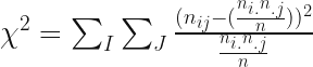 (1)
(1) is the total number of frequencies,
  is the letter frequency in row
  and column
  , and
, and  and
and  are the total frequencies in row
 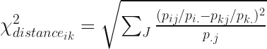 (2)
(2) , which is simply every entry in correspondenceMatrix (i.e. letter frequencies normalised by the grand total). dfchiSquaredDistances contains:
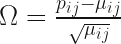 (3)
(3)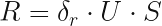 (4)
(4) and
and  are the left singular vectors matrix and singular values on the diagonal matrix from SVD. The
  is diagonal matrix made of the reciprocals of the square roots of the row totals.


