Greetings, my blog readers!
This is my first post in 2018. In this post I will share with you a very simple way of performing inference using Approximate Bayesian Computation (ABC) – not to be confused with Approximate Bootstrap Confidence interval, which is also “ABC”.
Let’s say we have observed some data, and are interested to test if there was a change in behaviour in whatever generated the data. For example, we could be monitoring the total amount that is spent/transferred from some account, and we would like to see if there was a shift in how much is being spent/transferred. Figure below shows what the data could look like. After we have eye-balled the graph, we think that all observations after item 43 belong to the changed behaviour (cutoff=43), and we separate the two by colour.

The first question that we can ask is about the means of the blue and the red regions: are they the same? In the figure above I am showing the mean and standard deviations for the two sets. We can run a basic bootstrap with replacement to check if the difference in the means is possibly accidental.

In the figure above basic_bootstrap generates a distribution of means of randomly sampled sets. The confidence interval is first computed as non-parametric. But a quick comparison with 95th CI using normal standard scores shows that the simulated and the non-simulated confidence intervals around the means are very close. Most importantly, the confidence intervals for the blue and red region means overlap, and thus we would have to accept the null hypothesis that the population means are the same and differences seen here are accidental.
Note how unsatisfying this result is. If we use some other test, like one-way ANOVA from scipy.stats.f_oneway, we get a p-value that is too high to accept an alternative hypothesis. However, if we plot the CDFs of the blue and the red data, we can clearly see that larger values are prevailing in the latter:

Approximate Bayesian Computation
Approximate Bayesian Computation (ABC) relates to probabilistic programming methods and allows us to quantify uncertainty more exactly than a simple CI. A pretty good summary of ABC can be found on Wikipedia. If we are monitoring transactions occurring over time, we may be interested in generating alerts when an amount is above a threshold (for example, your bank could have a monitoring system in place to safeguard you against credit card fraud). If, instead of comparing means of red and blue region, we decided to answer the question about how likely are we to see more trades above the threshold in the red vs. the blue data regions, we could use ABC.
To execute an ABC test on the difference in the number of trades above a threshold in the blue and red data regions, we begin by choosing the threshold! Take a look at the CDF plot above. We see that approximately half of red data is above 20. Whereas only 25% of blue data is above 20. Let’s set our threshold at 20. The ABC is a simple simulation algorithm where we repeatedly perform sample and compare steps. What can we sample here? We will sample from two normal distributions, each with the means set to the fraction of trades above our threshold. I will use Normal distribution, but it is purely a choice of convenience. Ok, what can we compare here? We will compare the number of trades that could have been above the threshold when the data they come from is sampled from the distributions we have chosen as our priors. And we store away the ones that are consistent with it. If we repeat this many times under the two parameterisations, we should build-up two distributions that can be used to answer the main question – how likely are we to obtain more trades above the chosen threshold in the red vs. the blue data sets. The code below does exactly that.

We obtain a very high probability of seeing more trades above the threshold in the red vs. the blue region.
 and
and  , the proportional change is:
 . In contrast, absolute moves are defined simply as the difference between two historical price observations:
  .
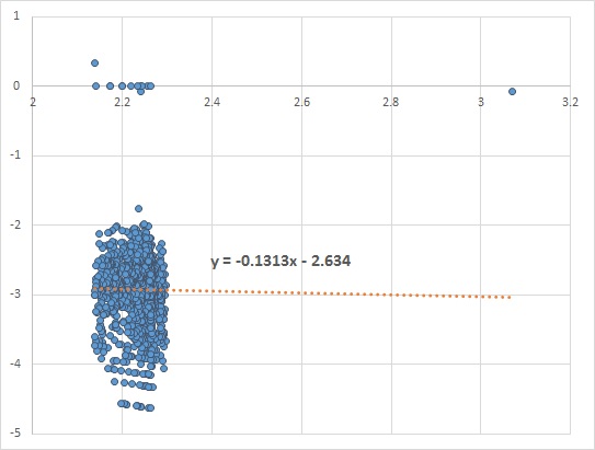
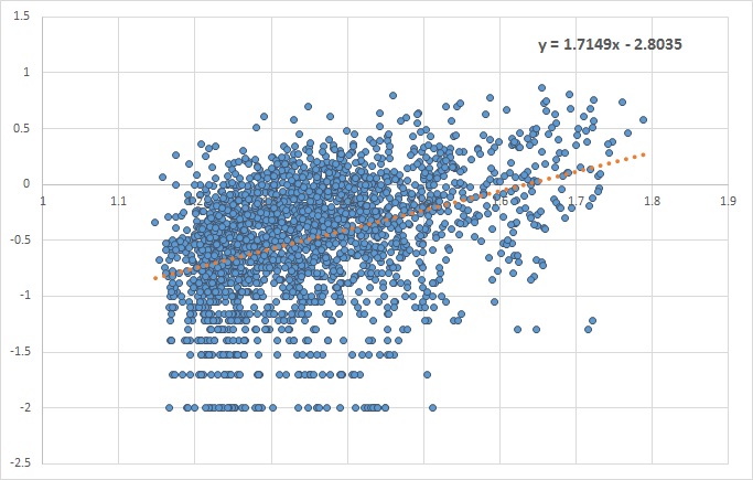
. vs.
vs.  we look for the value of the slope of the fitted linear line. A slope closer to zero indicates no dependency, while a positive or negative slope shows that the two variables are dependent.