
In this blog I will introduce the Correspondence Analysis – a visualisation technique for categorical data. All the code has been compiled in my github repository.
Correspondence Analysis (CA) has been around for a very long time. It was first developed in the 1930-ies, and made popular by M. Greenacre in the 1980-ies. It is an established statistical analysis techniques with dedicated annual symposiums and sufficient amount of literature covering theory and applications. Inspite of its popularity, I have only recently discovered it, and thought that it is worthwhile to document the fundamentals on my blog.
What Exactly is Correspondence Analysis?
CA is a visualisation technique that can be applied to categorical data for data exploration. Unlike numerical data, categorical features are harder to analyse and visualise. CA uses a matrix decomposition method, namely SVD, and thus you may see CA being likened to the Principle Components Analysis (PCA). However, CA is not, strictly speaking, a PCA for categorical data, mostly because the primary objective of CA is to provide a visualisation of associations among categorical features.
How does one visualise categorical data? CA is based on a simple concept of a contingency table. A contingency table is a tabulation of frequencies of how categorical values are distributed by variables. This blog will be using examples from P. Yelland’s article on CA published in the Mathematica journal[1]. I will translate his Mathematica code to Python (because Python is awesome). In [1] we find CA applied to textual analysis where passages of a few authors analysed by the frequency of letters. The five authors and the letters are shown below:
authors = ["Charles Darwin", "Rene Descartes","Thomas Hobbes", "Mary Shelley", "Mark Twain"]
initials=['CD1','CD2','CD3','RD1','RD2','RD3','TB1','TB2','TB3','MS1','MS2','MS3','MT1','MT2','MT3']
chars=["B", "C", "D", "F", "G", "H", "I", "L", "M", "N","P", "R", "S", "U", "W", "Y"]
The contingency table build from how often these letters appear in three passages per author are:
sampleCrosstab=[[34, 37, 44, 27, 19, 39, 74, 44, 27, 61, 12, 65, 69,22, 14, 21],
                [18, 33, 47, 24, 14, 38, 66, 41, 36,72, 15, 62, 63, 31, 12, 18],
                [32, 43, 36, 12, 21, 51, 75, 33, 23, 60, 24, 68, 85,18, 13, 14],
                [13, 31, 55, 29, 15, 62, 74, 43, 28,73, 8, 59, 54, 32, 19, 20],
                [8, 28, 34, 24, 17, 68, 75, 34, 25, 70, 16, 56, 72,31, 14, 11],
                [9, 34, 43, 25, 18, 68, 84, 25, 32, 76,14, 69, 64, 27, 11, 18],
                [15, 20, 28, 18, 19, 65, 82, 34, 29, 89, 11, 47, 74,18, 22, 17],
                [18, 14, 40, 25, 21, 60, 70, 15, 37,80, 15, 65, 68, 21, 25, 9],
                [19, 18, 41, 26, 19, 58, 64, 18, 38, 78, 15, 65, 72,20, 20, 11],
                [13, 29, 49, 31, 16, 61, 73, 36, 29,69, 13, 63, 58, 18, 20, 25],
                [17, 34, 43, 29, 14, 62, 64, 26, 26, 71, 26, 78, 64, 21, 18, 12],
                [13, 22, 43, 16, 11, 70, 68, 46, 35,57, 30, 71, 57, 19, 22, 20],
                [16, 18, 56, 13, 27, 67, 61, 43, 20, 63, 14, 43, 67,34, 41, 23],
                [15, 21, 66, 21, 19, 50, 62, 50, 24, 68, 14, 40, 58, 31, 36, 26],
                [19, 17, 70, 12, 28, 53, 72, 39, 22, 71, 11, 40, 67,25, 41, 17]]
Can you spot any differences in the use of letters by author from sampleCrosstab? It is almost impossible to do so by just looking at it. Instead, CA resorts to the 
Chi-Squared Statistic and Chi-Squared Distances
Pearson’s
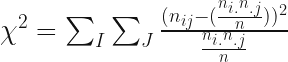
Where 


grandTotal = np.sum(sampleCrosstab)
correspondenceMatrix = np.divide(sampleCrosstab,grandTotal)
rowTotals = np.sum(correspondenceMatrix, axis=1)
columnTotals = np.sum(correspondenceMatrix, axis=0)

independenceModel = np.outer(rowTotals, columnTotals)

#Calculate manually
chiSquaredStatistic = grandTotal*np.sum(np.square(correspondenceMatrix-independenceModel)/independenceModel)
print(chiSquaredStatistic)

# Quick check - compare to scipy Chi-Squared test
statistic, prob, dof, ex = chi2_contingency(sampleCrosstab)
print(statistic)
print(np.round(prob, decimals=2))
In the above code correspondenceMatrix holds normalised frequencies. The
For the purposes of CA, the differences between the distributions of letters in the text samples are measured by
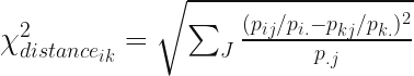
# pre-calculate normalised rows
norm_correspondenceMatrix = np.divide(correspondenceMatrix,rowTotals[:, None])

chiSquaredDistances = np.zeros((correspondenceMatrix.shape[0],correspondenceMatrix.shape[0]))

norm_columnTotals = np.sum(norm_correspondenceMatrix, axis=0)
for row in range(correspondenceMatrix.shape[0]):
    chiSquaredDistances[row]=np.sqrt(np.sum(np.square(norm_correspondenceMatrix
                                                        -norm_correspondenceMatrix[row])/columnTotals, axis=1))
# Save distances to the DataFrame
dfchiSquaredDistances = pd.DataFrame(data=np.round(chiSquaredDistances*100).astype(int), columns=authorSamples)

print(dfchiSquaredDistances)
In (2) I switched to notation with 

Chi-Squared Distances In Graphical Form
CA provides a means of representing a table of
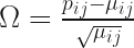
standardizedResiduals = np.divide((correspondenceMatrix-independenceModel),np.sqrt(independenceModel))

u,s,vh = np.linalg.svd(standardizedResiduals, full_matrices=False)
We are after the row scores, which are coordinates of points in a high-dimensional space (14 dimensions in this case). These points are arranged so that the Euclidean distance between two points is equal to the
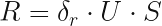
where 


deltaR = np.diag(np.divide(1.0,np.sqrt(rowTotals)))

rowScores=np.dot(np.dot(deltaR,u),np.diag(s))

dfFirstTwoComponents = pd.DataFrame(data=[l[0:2] for l in rowScores], columns=['X', 'Y'], index=initials)

print(dfFirstTwoComponents)
Extracting the first two components gives us:

Plotting these as points:

The plot clearly shows letters associations by author. Mark Twain and Charles Darwin’s samples stand out as significantly different from the rest.
Source and Reference: [1] P.Yelland, An Introduction to Correspondence Analysis. The Mathematica Journal 12, 2010 Wolfram Media, Inc.
