Transforming Uniform Random Variables to Normal

In my previous post here I have shared with you some methods for generating uniform random variables. For many practical tasks we need random variables that are distributed normally around some mean. There are two well know approaches for transforming uniform random variables to normal or Gaussian. These are – the inverse transform and the Box-Muller methods. Let’s take a look at each of them. I am also providing my version of C# implementation.

Inverse Transform Method

The general form of this method is:

X=F^{-1} (U),U\approx Unif[0,1]

Here U is a uniform random variable from [0,1] interval, F^{-1} is the inverse of the cumulative distribution function (i.e. any given c.d.f.), and X is the desired random variable satisfying P(X \leq x)=F(x) property. Again, the c.d.f. can be for any required distribution for which the inverse is well-defined.

To make sense of this method and to see why it works, let’s take a look at the graph of a normal c.d.f. where X \approx N(0,1). Figure 1 shows the probability on the y-axis and the random variable on the x-axis. The probability axis corresponds to the uniform random variable range, which is [0,1]. Thus, we can use the y-axis to map to the x-axis, which would give us a random variable in (-3,3) interval. This random variable is normally distributed with mean 0 and standard deviation of 1. In Figure 1 I have marked the middle of both axis to make it clear that uniform random variables between 0 and 0.5 would map to normal random variables that are negative. The uniforms above 0.5 map to positive r.vs.

Figure 1
Figure 1

I hope by now it is clear how the inverse transform method works. The main reason it always works for a well-behaved distribution like the normal distribution is because the ‘mapping’ is one-to-one. That is, for each value of U, we have a unique mapping onto X. A good intuitive way to think about the inverse transform method is by analogy to taking a percentile of some distribution.

The standard normal cumulative distribution function is:

F(x)=\frac{1}{\sqrt{2\pi}} \int_{-\infty}^{x} \exp{\frac{-u^{2}}{2}} du

To use the inverse transform method we need to take the inverse, or calculate F^{-1}, for which an exact solution is not achievable computationally, and we will need to approximate it. Several numerical approximations can be found in the relevant literature. Check out, for example chapter 2.3.2 in [1] or on the Wikipedea. I will demonstrate two approximations of two different levels of accuracy.

In [1] we find a summary of the rational approximation proposed by Beasley and Springer:

F^{-1} (x) \approx \frac{\sum_{n=0}^{3} a_n (x-\frac{1}{2})^{(2n+1)}}{1+\sum_{n=0}^{3} b_n (x-\frac{1}{2})^{2n}}

Where a_n and b_n are constants (see the code for their values). The above is defined for 0.5 \le x \le0.92. For x > 0.92, we can utilize Chebyshev’s approximation, as demonstrated in [1]:

F^{-1} (x) \approx \sum_{n=0}^{8} c_n (\log(-\log(1-x)))^{n} ,0.92 \leq x<1

The values below 0.5 can be derived by symmetry. The above method gives a high accuracy with a maximum absolute error of 3*10^{-9} over the [-7,7] range for x.

A less accurate method involves approximating the error function erf, since the inverse c.d.f. can be defined in terms of erf as follows:

F^{-1} (x)=\sqrt{2} \cdot erf^{-1} (2x-1)

The inverse error function can be approximated using:

erf^{-1} (x) \approx sign(x) \sqrt{\theta}

\theta =\sqrt{{\left(\frac{2}{\pi\alpha}+\frac{ln(1-x^{2})}{2}\right)}^{2}-\frac{ln(1-x^{2})}{\alpha}}-\frac{2}{\pi\alpha}+\frac{ln(1-x^{2})}{2}

\alpha =\frac{8(\pi-3)}{3\pi(4-\pi)}

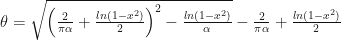
This approach achieves a maximum absolute error of 0.00035 for all x. To me, the erf method is simpler, both, to understand and to implement.

Box-Muller Method

Box-Muller method for transforming uniform random variables to normal r.vs. is an algorithms that involves choosing a random point uniformly from the circle of radius \sqrt{R}, such that R=Z_1^{2}+Z_2^{2} follows exponential distribution with mean 2 and Z_n\sim N_2 (0,I_2 ) (i.e. bivariate normal).

Box-Muller method requires two uniform random variables, and it produces two standard normal random variables. The reason for having two, is because we are simulating a point on a circle in x,y plane. So, to pick a random point on a circle we need a radius and the angle it makes with the origin. If we can randomise the radius and the angle with the origin (using the two random uniforms), we can achieve a random way of simulating the (x,y) point on a circle. Take a look at Figure 2 below, which demonstrates this concept.

Figure 2
Figure 2

Ok, hopefully the above gives you a clear explanation for the foundations of the inverse transform and the Box-Muller methods. Let’s now look at how we can implement them in C#.

Implementation

Box-Muller class has an overloaded method that works for a single pair or a 2D array of r.v.s:

internal sealed class BoxMuller
    {
        /// <summary>
        /// Returns an arrays with Z1 and Z2 - two standard normal random variables generated using Box-Muller method
        /// </summary>
        /// <param name="U1">first standard random uniform</param>
        /// <param name="U2">second standard randoom uniform</param>
        /// <returns>double[] of length=2</returns>
        internal double[] BoxMullerTransform(double U1, double U2)
        {
            double[] normals = new double[2];
            if (U1 < 0 || U1 > 1 || U2 < 0 || U2 > 1)
            {
                normals[0] = default(double);
                normals[1] = default(double);
            }
            else
            {
                double sqrtR = Math.Sqrt(-2.0*Math.Log(U1));
                double v = 2.0*Math.PI*U2;

                normals[0] = sqrtR * Math.Cos(v);
                normals[1] = sqrtR * Math.Sin(v);
            }
            return normals;
        }

        /// <summary>
        /// Returns a 2D array with Z1[] and Z2[] - two standard normal random variables generated using Box-Muller method
        /// </summary>
        /// <param name="U1">u1[] an array of first standard random uniforms</param>
        /// <param name="U2">u2[] an array of second standard random uniforms</param>
        /// <returns>double[L,2] of L=min(Length(u1),Length(u2))</returns>
        internal double[,] BoxMullerTransform(double[] U1, double[] U2)
        {
            long count=U1.Length<=U2.Length?U1.Length:U2.Length;

            double[,] normals = new double[count, 2];
            double u1, u2;

            for (int i = 0; i < count; i++)
            {
                u1 = U1[i];
                u2 = U2[i];
                if (u1 < 0 || u1 > 1 || u2 < 0 || u2 > 1)
                {
                    normals[i,0] = default(double);
                    normals[i,1] = default(double);
                }
                else
                {
                    double sqrtR = Math.Sqrt(-2.0 * Math.Log(u1));
                    double v = 2.0 * Math.PI * u2;

                    normals[i,0] = sqrtR * Math.Cos(v);
                    normals[i,1] = sqrtR * Math.Sin(v);
                }
            }
            return normals;
        }
    }

The inverse transform has four internal methods for generating normal r.v.s. As described before, the ERF method is simpler, and is also easier to implement. The Beasley-Springer-Moro (BSM) method is based on the algorithm found in [1], pg. 68. I’ve verified that it gives an accurate solution up to 9.d.p. Note that InverseTransformERF is an approximation to InverseTransformMethod, and it seems to achieve an accuracy of up to 4 d.p.

internal sealed class InverseTransform
    {
        /// <summary>
        /// Returns a standard normal random variable given a standard uniform random variable
        /// </summary>
        /// <param name="x">standard uniform rv in [0,1]</param>
        /// <returns>standard normal rv in (-3,3)</returns>
        internal double InverseTransformMethod(double x)
        {
            if (x < 0 || x > 1)
                return default(double);
            
            double res,r;
            double y = x - 0.5;
            if(y<0.42)
            {
                r = y * y;
                res = y * (((a3 * r + a2) * r + a1) * r + a0) / ((((b3 * r + b2) * r + b1) * r + b0) * r + 1.0);
            }
            else
            {
                r = (y > 0) ? (1 - x) : x;
                r = Math.Log(-1.0 * Math.Log(r));
                res = c0 + r * (c1 + r * (c2 + r * (c3 + r * (c4 + r * (c5 + r * (c6 + r * c7 + r * c8))))));
                res = (y < 0) ? -1.0 * res : res;
            }
            return res;
        }
        /// <summary>
        /// Returns an array of standard normal random variables given an array of standard uniform random variables
        /// </summary>
        /// <param name="x">an array of doubles: uniform rvs in [0,1]</param>
        /// <returns>an array of doubles: standard normal rvs in (-3,3)</returns>
        internal double[] InverseTransformMethod(double[] x)
        {
            long size = x.Length;
            double[] res = new double[size];
            double r,y;


            for (int i = 0; i < size;i++)
            {
                if (x[i]<0 || x[i]>1)
                {
                    res[i] = 0;
                    continue;
                }

                y = x[i] - 0.5;
                if (y < 0.42)
                {
                    r = y * y;
                    res[i] = y * (((a3 * r + a2) * r + a1) * r + a0) / ((((b3 * r + b2) * r + b1) * r + b0) * r + 1.0);
                }
                else
                {
                    r = (y > 0) ? (1 - x[i]) : x[i];
                    r = Math.Log(-1.0 * Math.Log(r));
                    res[i] = c0 + r * (c1 + r * (c2 + r * (c3 + r * (c4 + r * (c5 + r * (c6 + r * c7 + r * c8))))));
                    res[i] = (y < 0) ? -1.0 * res[i] : res[i];
                }
            }
            return res;
        }
        /// <summary>
        /// Performs an inverse transform using erf^-1
        /// Returns a standard normal random variable given a standard uniform random variable
        /// </summary>
        /// <param name="x">standard uniform rv in [0,1]</param>
        /// <returns>standard normal rv in (-3,3)</returns>
        internal double InverseTransformERF(double x)
        {
            return Math.Sqrt(2.0) * InverseErf(2.0 * x - 1);
        }

        /// <summary>
        /// Performs an inverse transform using erf^-1
        /// Returns an array of standard normal random variables given an array of standard uniform random variables
        /// </summary>
        /// <param name="x">an array of doubles: uniform rvs in [0,1]</param>
        /// <returns>an array of doubles: standard normal rvs in (-3,3)</returns>
        internal double[] InverseTransformERF(double[] x)
        {
            long size = x.Length;
            double[] res = new double[size];
            for (int i = 0; i < size; i++ )
            {
                res[i] = Math.Sqrt(2.0) * InverseErf(2.0 * x[i] - 1);
            }
                return res;
        }

        private double InverseErf(double x)
        {
            double res;
            double K = scalor + (Math.Log(1 - x * x)) / (2.0);
            double L=(Math.Log(1-x*x))/(alpha);
            double T = Math.Sqrt(K*K - L);

            res = Math.Sign(x) * Math.Sqrt(T-K);
            return res;
        }

        //used by the ERF method
        private const double alpha = (8.0 * (Math.PI - 3.0)) / (3.0 * Math.PI * (4.0 - Math.PI));
        private const double scalor = (2.0) / (Math.PI * alpha);

        //used by the BSM method in "Monte Carlo Methods in Financial Engineering" by P.Glasserman
        //note that a double achieves 15-17 digit precision
        //since these constancts are small, we are not using decimal type
        private const double a0 = 2.50662823884;
        private const double a1 = -18.61500062529;
        private const double a2 = 41.39119773534;
        private const double a3 = -25.44106049637;
        private const double b0 = -8.47351093090;
        private const double b1 = 23.08336743743;
        private const double b2 = -21.06224101826;
        private const double b3 = 3.13082909833;
        private const double c0 = 0.3374754822726147;
        private const double c1 = 0.9761690190917186;
        private const double c2 = 0.16079797149118209;
        private const double c3 = 0.0276438810333863;
        private const double c4 = 0.0038405729373609;
        private const double c5 = 0.0003951896511919;
        private const double c6 = 0.0000321767881768;
        private const double c7 = 0.0000002888167364;
        private const double c8 = 0.0000003960315187;

    }

Surely the two different methods map the uniforms to different normal r.v.s. So, how can we compare these two methods? One way would be to consider simplicity, speed and the accuracy vs. the exact solution.

References:
[1]P. Glasserman. “Monte Carlo Methods in Financial Engineering”, 2004. Springer-Verlag.

Random Numbers Generator

At the heart of any Monte Carlo method are two fundamental building blocks. The first is the generation of uniform random variables. The second is the transformation of the generated uniform distribution to whichever is the required distribution for the task at hand. For example, a normal one. The quality of random number generator determines the quality of the final distribution.

No matter how good is the underlying random number generation algorithm, the outcome is not truly random, since the algorithm that produces the numbers is fully deterministic. In fact, I actually believe that very few things in live are truly random. Even the seemingly random roulette wheel is influenced by the physical properties such as friction, weight and skewness. So, let’s embrace the fact that we’ll only ever be able to achieve pseudo-randomness. This should be good enough for all practical purposes. Thus, I will stop using ‘pseudo-random’, and use the word ‘random’ instead.

In this post I will show you some very basic algorithms for generating random numbers. If you do further research, you will find that the more complex algorithms are extensions of the basic ones.

Take int x = 1. We can use x to generate a next random number. How? Well, take, for example:

x_next = (25,173*x+13,849) %201

where % is the modulus operator. x_next is (also an integer) = 28. Ok, 28 is kind-of random. Let’s repeat the above calculation where x=28. x_next becomes 118. Hm, if I keep repeating the same ‘substitute/calculate’ steps 10 times, I get:

28, 118, 16, 145, 106, 43, 34, 4, 172, 196

Well, that looks pretty random to me! I use this algorithm to generate 200 integers and show them in Figure 1 (hint: click on it to see the details).

Figure 1
Figure 1

Before I point out a problem with this random sample, let me explain what is going on here. The way I generated my random variables is called linear congruential generator, originally introduced by D.H.Lehmer in 1951. It has a general form of

x_{i+1}=(a \times x_{i}+c) \mod{m}

The above will produce a sequence of random numbers in the region between 1 and m-1. If the required uniform variables should be in the unit interval, we can scale by 1/m. Referring back to our initial example, a, c and m are some constants. It turns out that the values of these constants are critical in determining the quality of the generated random variable sequence. Looking at Figure 1 you should be able to spot that the random sequence repeats itself exactly after only 65 iterations. Clearly, this is not a very good random number generator! Ideally, we need an algorithm that can simulate all m-1 random variables without repeating itself. This condition is known as ‘having a full period length’, and it is one of the standard criteria for selecting a random number generator.

In (1), we find the list of conditions a, c and m must satisfy to ensure we obtain a full period length (if c!=0):

  • c and m are relatively prime (their only common divisor is 1);
  • every prime number that divides m, also divides a-1;
  • a-1 is divisible by 4, if m is;

So, the reason we did not obtain the full period length is because the chosen constants do not meet these conditions. If we change m to be 217, it allows for a full period of length 216.

The demonstrated random number generator is the basis for more complex generators. A good random number generator should be able to generate millions of numbers without repeating the sequence. If we are to stick to the int representation, we have to take care not to overflow. Reminder: a System.Int32 variable can hold a maximum value of [(2^32)-1]/2-1.

Many various extensions to the linear congruential generator have been developed over the years; many involving a combination of several linear ones which result in a much longer period length. In C#, the System.Random class provides an easy way to generate random variables. The full implementation of this class can be found here. Random class can be initialised with a given seed, or without. When no seed is provided, the default seed is Environment.TickCount, which is the time in milliseconds since the computer been booted-up. The algorithm behind System.Random is based on the routine in “Numerical Recipes In C: The Art Of Scientific Computing”, which, according to the authors, has been proposed by D.Knuth. The algorithm has elements of the linear congruential generator, but is essentially a mixed ‘subtractive method’ where an array of 55 pseudo-random integers is maintained. At the class initialization, the array is populated with values twice. First, the array is populated with values between 0 and [max(System.Int32)-1]. At this point, the index of the array which receives the value is selected using

x=(21 \times i)\mod{55}

This is ‘the element’ of the linear congruential generator I’ve mentioned above. Here i is in [1,54]. Note that c is set to zero, and the three conditions listed above do not apply. The second time the array is re-populated, it’s values are further randomized by cycling through the array four times and reassigning each value with a difference between its original value and a value at another index, which is approximately half-the-array length away. Positivity is ensured by adding max(System.Int32) to any negative number.

Every time a user asks for the next random number, the difference between two values in the array is returned. At the same time, one of the values in the array is replaced with the value returned to the user. There is a check for positivity, which is ensured by adding max(System.Int32) to any negative number.

The Random class has additional methods to allow for simulating random numbers in some range or even simulating random doubles. The latter returns a a double equal to a randomly generated integer scaled by (1/ max(System.Int32)).

 
References:
(1) P. Glasserman. “Monte Carlo Methods in Financial Engineering”, 2004. Springer-Verlag.

Monte Carlo Methods

Monte Carlo is a name given to numerical methods that involve random number generation. Such numerical methods are used to solve many problems in mathematics, finance and computing. For example, simulation of a random walk is based on some Monte Carlo algorithm. Also, sampling from a subset of a large data set in order to deduce the data set properties is another application of Monte Carlo. In my Monte Carlo posts I will cover random number generation techniques, simulation of price paths of financial assets and other interesting topics.