This is my first post in 2018. In this post I will share with you a very simple way of performing inference using Approximate Bayesian Computation (ABC) – not to be confused with Approximate Bootstrap Confidence interval, which is also “ABC”.
Let’s say we have observed some data, and are interested to test if there was a change in behaviour in whatever generated the data. For example, we could be monitoring the total amount that is spent/transferred from some account, and we would like to see if there was a shift in how much is being spent/transferred. Figure below shows what the data could look like. After we have eye-balled the graph, we think that all observations after item 43 belong to the changed behaviour (cutoff=43), and we separate the two by colour.
The first question that we can ask is about the means of the blue and the red regions: are they the same? In the figure above I am showing the mean and standard deviations for the two sets. We can run a basic bootstrap with replacement to check if the difference in the means is possibly accidental.
In the figure above basic_bootstrap generates a distribution of means of randomly sampled sets. The confidence interval is first computed as non-parametric. But a quick comparison with 95th CI using normal standard scores shows that the simulated and the non-simulated confidence intervals around the means are very close. Most importantly, the confidence intervals for the blue and red region means overlap, and thus we would have to accept the null hypothesis that the population means are the same and differences seen here are accidental.
Note how unsatisfying this result is. If we use some other test, like one-way ANOVA from scipy.stats.f_oneway, we get a p-value that is too high to accept an alternative hypothesis. However, if we plot the CDFs of the blue and the red data, we can clearly see that larger values are prevailing in the latter:
Approximate Bayesian Computation
Approximate Bayesian Computation (ABC) relates to probabilistic programming methods and allows us to quantify uncertainty more exactly than a simple CI. A pretty good summary of ABC can be found on Wikipedia. If we are monitoring transactions occurring over time, we may be interested in generating alerts when an amount is above a threshold (for example, your bank could have a monitoring system in place to safeguard you against credit card fraud). If, instead of comparing means of red and blue region, we decided to answer the question about how likely are we to see more trades above the threshold in the red vs. the blue data regions, we could use ABC.
To execute an ABC test on the difference in the number of trades above a threshold in the blue and red data regions, we begin by choosing the threshold! Take a look at the CDF plot above. We see that approximately half of red data is above 20. Whereas only 25% of blue data is above 20. Let’s set our threshold at 20. The ABC is a simple simulation algorithm where we repeatedly perform sample and compare steps. What can we sample here? We will sample from two normal distributions, each with the means set to the fraction of trades above our threshold. I will use Normal distribution, but it is purely a choice of convenience. Ok, what can we compare here? We will compare the number of trades that could have been above the threshold when the data they come from is sampled from the distributions we have chosen as our priors. And we store away the ones that are consistent with it. If we repeat this many times under the two parameterisations, we should build-up two distributions that can be used to answer the main question – how likely are we to obtain more trades above the chosen threshold in the red vs. the blue data sets. The code below does exactly that.
We obtain a very high probability of seeing more trades above the threshold in the red vs. the blue region.
It will be a safe assumption to make that people who read my blogs work with data. In finance, the data is often in form of asset prices or other market indicators like implied volatility. Analyzing price data often requires calculating returns (aka. moves). Very often we work with proportional returns or log returns. Proportional returns are calculated relative to the price level. For example, given any two historical prices and , the proportional change is:
The above can be shortened as . In contrast, absolute moves are defined simply as the difference between two historical price observations: .
How do you know which type of return is appropriate for your data? The answer depends on the price dynamic and the simulation/analysis task at hand. Historical simulation, often used in Value-at-Risk (VaR), requires calculating PnL strip from some sensitivity and a set of historical returns. For example, a VaR model for foreign exchange options may be specified to take into account PnL impact from changes in implied volatility skew. Here, the PnL is historically simulated using sensitivities of a volatility curve or surface and historical implied volatility returns for some surface parameter, like low risk reversal. You have a choice in how to calculate the volatility returns. The right choice can be determined with a simple regression.
Essentially, we need to look for evidence of dependency of price returns on price levels. In FX, liquid options on G21 currency pairs do not exhibit such dependency, while emerging market pairs do. I have not been able to locate a free source of implied FX volatility, but I have found two instruments that are good enough to demonstrate the concept. CBOE LOVOL Index is a low volatility index and can be downloaded for free from Quandl. For this example I took the close of day prices from 2012-2017. After plotting vs. we look for the value of the slope of the fitted linear line. A slope closer to zero indicates no dependency, while a positive or negative slope shows that the two variables are dependent.
CBOE LVOL
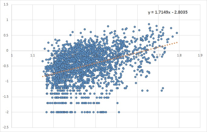
In the absence of dependency, absolute returns can be used, while proportional return are otherwise more appropriate. Take a look at a plot of VXMT CBOE Mid-term Volatility Index. The fitted linear line has a slope of approximately 1.7. Historical simulation of VXMT is calling for proportional rather than absolute price moves.
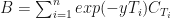
In fixed income analysis it is often required to calculate the yield of some coupon paying instrument, for example a bond. Very simply, an yield of a bond is defined as a single rate of return. Under continuous compounding, given a set of interest rates , the yield equates the present value of the bond computed under a given set of rates. In other words:
where is a coupon paid out at time . Usually, one solves for using some iterative guess-work, e.g. goal seek. In this post I will show you a well-know Newton’s recursive method that can be used to base such goal seek on.
The Newton’s Method
The Newton’s method is based on a recursive approximation formula:
Let be the price(or present value) of the bond expressed via its yield. Then, taking to represent interest rate, we have: and
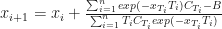
The recursive formula to solve for yield becomes:
Goal Seek in C#
Now let’s take a look at an example implementation. The while loop in CalculateYield method implements the goal seek. This is a very simple example, and we pretend to have the bond price.
using System;
using System.Collections.Generic;
using System.Linq;

namespace YieldCalculator
{
    class EntryPoint
    {
        static void Main(string[] args)
        {
            // use some numbers to illustrate the point
            // maturities in months
            int[] maturities = { 6, 12, 18, 24, 30, 36 };
            double[] yearFrac = maturities.Select(i => i / 12.0).ToArray();
            // bond principle
            double P = 100;
            // bond price
            double B = 108;
            double couponRate = 0.1;
            // calculate future cashflows
            double[] cashflows = maturities.Select(i => (P * couponRate) / 2.0).ToArray();
            // add principle repayment
            cashflows[cashflows.Count() - 1] = P + cashflows[cashflows.Count() - 1];

            double initialGuess = 0.1;
            Console.WriteLine(CalculateYield(initialGuess, cashflows, yearFrac, B));
        }

        static double CalculateYield(double initialGuess, double[] cashflows, double[] yearFrac, double B)
        {
            double error = 0.000000001;
            double x_i = initialGuess-1.0;
            double x_i_next = initialGuess;

            double numerator;
            double denominator;

            while (Math.Abs(x_i_next - x_i) > error)
            {
                x_i = x_i_next;
                // linq's Zip is handy to perform a sum over expressions involving several arrays
                numerator = cashflows.Zip(yearFrac, (x,y) => (x * Math.Exp(y *-1*x_i))).Sum();
                denominator = yearFrac.Zip(cashflows, (x,y) => (x*y*Math.Exp(x*-1*x_i))).Sum();
                x_i_next = x_i + (numerator - B) / denominator;
            }
            return x_i_next;
        }
    }
}
Note how handy is LINQ’s Zip function to calculate a sum over an expression involving two arrays.
And now to the burning question – why the picture of a cat? The answer is even simpler than this post: It is a cute cat, so, why not?
In this post on numerical methods I will share with you the theoretical background and the implementation of the two types of interpolations: linear and natural cubic spline. These interpolations are often used within the financial industry. For example, discount rates for some maturity for which there is no point on an yield curve is often interpolated using cubic spline interpolation. Another example can be in risk management, like a position’s Value-at-Risk calculation obtained from a partial or a 2-dimensional revaluation grid.
Linear Interpolation
Let’s begin with the simplest method – linear interpolation. The idea is that we are given a set of numerical points and function values at these points. The task is to use the given set and approximate the function’s value at some different points. That is, given where our task is to estimate for . Of course we may require to go outside of the range of our set of points, which would require extrapolation (or projection outside the known function values).
Almost all interpolation techniques are based around the concept of function approximation. Mathematically, the backbone is simple:
The above expression tells us that the value of the function we are approximating at point x will be around and that . We can re-write this expression as follows:
where we have substituted for and for . Our linear interpolation is now taking a form of linear regression around .
Linear interpolation is the most basic type of interpolations. It works remarkably well for smooth functions with sufficient number of points. However, because it is such a basic method, interpolating more complex functions requires a little bit more work.
Cubic Spline Interpolation
In what follows I am going to borrow a few formulations from a very good book: Guide to Scientific Computing by P.R.Turner. The idea of a spline interpolation is to extend the single polynomial of linear interpolation to higher degrees. But unlike with piece-wise polynomials, the higher degree polynomials constructed by the cubic spline are different in each interval . The cubic spline can be defined as:
If you compare the above expression with the linear interpolation, you will see that we have added two terms to the rhs. It is these extra terms that should allow us achieve greater precision. There are certain requirements placed on s. These are: it must be continuous, and its first and second derivatives must exist. We only need to determine and coefficients, since . Take . The continuity condition (see P.R.Turner pg. 104) gives the following equalities:
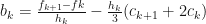
Thus, if we had the values for , we would be able to determine all the coefficients. After some re-arranging, it is possible to obtain:
for . This is a tridiagonal system of linear equations, which can be solved in a number of ways.
Let’s now look at how we can implement the linear and cubic spline interpolation in C#.
Implementing Linear and Cubic Spline Interpolation in C#
The code is broken into five regions. Tridiagonal Matrix region defines a Tridiagonal class to solve a system of linear equations. The Extensions regions defines a few extensions to allows for matrix manipulations. The Foundation region is where the parent Interpolation class is defined. Both, Linear and Cubic Spline Interpolations classes inherit from it.
using System;
using System.Collections;
using System.Collections.Generic;
using System.Linq;
using System.Text;
using System.Threading.Tasks;
namespace TridiagonalMatrix
{
#region TRIDIAGONAL_MATRIX
// solves a Tridiagonal Matrix using Thomas algorithm
public sealed class Tridiagonal
{
public double[] Solve(double[,] matrix, double[] d)
{
int rows = matrix.GetLength(0);
int cols = matrix.GetLength(1);
int len = d.Length;
// this must be a square matrix
if (rows == cols && rows == len)
{
double[] b = new double[rows];
double[] a = new double[rows];
double[] c = new double[rows];
// decompose the matrix into its tri-diagonal components
for (int i = 0; i < rows; i++)
{
for (int j=0; j<cols; j++)
{
if (i == j)
b[i] = matrix[i, j];
else if (i == (j - 1))
c[i] = matrix[i, j];
else if (i == (j + 1))
a[i] = matrix[i, j];
}
}
try
{
c[0] = c[0] / b[0];
d[0] = d[0] / b[0];
for (int i = 1; i < len - 1; i++)
{
c[i] = c[i] / (b[i] - a[i] * c[i - 1]);
d[i] = (d[i] - a[i] * d[i - 1]) / (b[i] - a[i] * c[i - 1]);
}
d[len - 1] = (d[len - 1] - a[len - 1] * d[len - 2]) / (b[len - 1] - a[len - 1] * c[len - 2]);
// back-substitution step
for (int i = (len - 1); i-- > 0; )
{
d[i] = d[i] - c[i] * d[i + 1];
}
return d;
}
catch(DivideByZeroException)
{
Console.WriteLine("Division by zero was attempted. Most likely reason is that ");
Console.WriteLine("the tridiagonal matrix condition ||(b*i)||>||(a*i)+(c*i)|| is not satisified.");
return null;
}
}
else
{
Console.WriteLine("Error: the matrix must be square. The vector must be the same size as the matrix length.");
return null;
}
}
}
#endregion
}
namespace BasicInterpolation
{
#region EXTENSIONS
public static class Extensions
{
// returns a list sorted in ascending order
public static List<T> SortedList<T>(this T[] array)
{
List<T> l = array.ToList();
l.Sort();
return l;
}
// returns a difference between consecutive elements of an array
public static double[] Diff(this double[] array)
{
int len = array.Length - 1;
double[] diffsArray = new double[len];
for (int i = 1; i <= len;i++)
{
diffsArray[i - 1] = array[i] - array[i - 1];
}
return diffsArray;
}
// scaled an array by another array of doubles
public static double[] Scale(this double[] array, double[] scalor, bool mult=true)
{
int len = array.Length;
double[] scaledArray = new double[len];
if (mult)
{
for (int i = 0; i < len; i++)
{
scaledArray[i] = array[i] * scalor[i];
}
}
else
{
for (int i = 0; i < len; i++)
{
if (scalor[i] != 0)
{
scaledArray[i] = array[i] / scalor[i];
}
else
{
// basic fix to prevent division by zero
scalor[i] = 0.00001;
scaledArray[i] = array[i] / scalor[i];
}
}
}
return scaledArray;
}
public static double[,] Diag(this double[,] matrix, double[] diagVals)
{
int rows = matrix.GetLength(0);
int cols = matrix.GetLength(1);
// the matrix has to be scare
if (rows==cols)
{
double[,] diagMatrix = new double[rows, cols];
int k = 0;
for (int i = 0; i < rows; i++)
for (int j = 0; j < cols; j++ )
{
if(i==j)
{
diagMatrix[i, j] = diagVals[k];
k++;
}
else
{
diagMatrix[i, j] = 0;
}
}
return diagMatrix;
}
else
{
Console.WriteLine("Diag should be used on square matrix only.");
return null;
}
}
}
#endregion
#region FOUNDATION
internal interface IInterpolate
{
double? Interpolate( double p);
}
internal abstract class Interpolation: IInterpolate
{
public Interpolation(double[] _x, double[] _y)
{
int xLength = _x.Length;
if (xLength == _y.Length && xLength > 1 && _x.Distinct().Count() == xLength)
{
x = _x;
y = _y;
}
}
// cubic spline relies on the abscissa values to be sorted
public Interpolation(double[] _x, double[] _y, bool checkSorted=true)
{
int xLength = _x.Length;
if (checkSorted)
{
if (xLength == _y.Length && xLength > 1 && _x.Distinct().Count() == xLength && Enumerable.SequenceEqual(_x.SortedList(),_x.ToList()))
{
x = _x;
y = _y;
}
}
else
{
if (xLength == _y.Length && xLength > 1 && _x.Distinct().Count() == xLength)
{
x = _x;
y = _y;
}
}
}
public double[] X
{
get
{
return x;
}
}
public double[] Y
{
get
{
return y;
}
}
public abstract double? Interpolate(double p);
private double[] x;
private double[] y;
}
#endregion
#region LINEAR
internal sealed class LinearInterpolation: Interpolation
{
public LinearInterpolation(double[] _x, double [] _y):base(_x,_y)
{
len = X.Length;
if (len > 1)
{
Console.WriteLine("Successfully set abscissa and ordinate.");
baseset = true;
// make a copy of X as a list for later use
lX = X.ToList();
}
else
Console.WriteLine("Ensure x and y are the same length and have at least 2 elements. All x values must be unique.");
}
public override double? Interpolate(double p)
{
if (baseset)
{
double? result = null;
double Rx;
try
{
// point p may be outside abscissa's range
// if it is, we return null
Rx = X.First(s => s >= p);
}
catch(ArgumentNullException)
{
return null;
}
// at this stage we know that Rx contains a valid value
// find the index of the value close to the point required to be interpolated for
int i = lX.IndexOf(Rx);
// provide for index not found and lower and upper tabulated bounds
if (i==-1)
return null;
if (i== len-1 && X[i]==p)
return Y[len - 1];
if (i == 0)
return Y[0];
// linearly interpolate between two adjacent points
double h = (X[i] - X[i - 1]);
double A = (X[i] - p) / h;
double B = (p - X[i - 1]) / h;
result = Y[i - 1] * A + Y[i] * B;
return result;
}
else
{
return null;
}
}
private bool baseset = false;
private int len;
private List<double> lX;
}
#endregion
#region CUBIC_SPLINE
internal sealed class CubicSplineInterpolation:Interpolation
{
public CubicSplineInterpolation(double[] _x, double[] _y): base(_x, _y, true)
{
len = X.Length;
if (len > 1)
{
Console.WriteLine("Successfully set abscissa and ordinate.");
baseset = true;
// make a copy of X as a list for later use
lX = X.ToList();
}
else
Console.WriteLine("Ensure x and y are the same length and have at least 2 elements. All x values must be unique. X-values must be in ascending order.");
}
public override double? Interpolate(double p)
{
if (baseset)
{
double? result = 0;
int N = len - 1;
double[] h = X.Diff();
double[] D = Y.Diff().Scale(h, false);
double[] s = Enumerable.Repeat(3.0, D.Length).ToArray();
double[] dD3 = D.Diff().Scale(s);
double[] a = Y;
// generate tridiagonal system
double[,] H = new double[N-1, N-1];
double[] diagVals = new double[N-1];
for (int i=1; i<N;i++)
{
diagVals[i-1] = 2 * (h[i-1] + h[i]);
}
H = H.Diag(diagVals);
// H can be null if non-square matrix is passed
if (H != null)
{
for (int i = 0; i < N - 2; i++)
{
H[i, i + 1] = h[i + 1];
H[i + 1, i] = h[i + 1];
}
double[] c = new double[N + 2];
c = Enumerable.Repeat(0.0, N + 1).ToArray();
// solve tridiagonal matrix
TridiagonalMatrix.Tridiagonal le = new TridiagonalMatrix.Tridiagonal();
double[] solution = le.Solve(H, dD3);
for (int i = 1; i < N;i++ )
{
c[i] = solution[i - 1];
}
double[] b = new double[N];
double[] d = new double[N];
for (int i = 0; i < N; i++ )
{
b[i] = D[i] - (h[i] * (c[i + 1] + 2.0 * c[i])) / 3.0;
d[i] = (c[i + 1] - c[i]) / (3.0 * h[i]);
}
double Rx;
try
{
// point p may be outside abscissa's range
// if it is, we return null
Rx = X.First(m => m >= p);
}
catch
{
return null;
}
// at this stage we know that Rx contains a valid value
// find the index of the value close to the point required to be interpolated for
int iRx = lX.IndexOf(Rx);
if (iRx == -1)
return null;
if (iRx == len - 1 && X[iRx] == p)
return Y[len - 1];
if (iRx == 0)
return Y[0];
iRx = lX.IndexOf(Rx)-1;
Rx = p - X[iRx];
result = a[iRx] + Rx * (b[iRx] + Rx * (c[iRx] + Rx * d[iRx]));
return result;
}
else
{
return null;
}
}
else
return null;
}
private bool baseset = false;
private int len;
private List<double> lX;
}
#endregion
class EntryPoint
{
static void Main(string[] args)
{
// code relies on abscissa values to be sorted
// there is a check for this condition, but no fix
// f(x) = 1/(1+x^2)*sin(x)
double[] ex = { -5, -3, -2, -1, 0, 1, 2, 3, 5};
double[] ey = { 0.036882, -0.01411, -0.18186, -0.42074, 0, 0.420735, 0.181859, 0.014112, -0.03688};
double[] p = {-5,-4.5,-4,-3.5,-3.2,-3,-2.8,-2.1,-1.5,-1,-0.8,0,0.65,1,1.3,1.9,2.6,3.1,3.5,4,4.5,5 };
LinearInterpolation LI = new LinearInterpolation(ex, ey);
CubicSplineInterpolation CS = new CubicSplineInterpolation(ex, ey);
Console.WriteLine("Linear Interpolation:");
foreach (double pp in p)
{
Console.Write(LI.Interpolate(pp).ToString()+", ");
}
Console.WriteLine("Cubic Spline Interpolation:");
foreach (double pp in p)
{
Console.WriteLine(CS.Interpolate(pp).ToString());
}
Console.ReadLine();
}
}
}
Note that I wrote a console application, and this is the reason for throwing as few exceptions as possible. Like with all the code on my blog – please feel free to take it and modify as you wish. It is now time to compare performance of linear and cubic spline interpolations on a test function: . Using the above code we obtain the following results:
In this post I will share with you a lazy way to expose boost.math library to a C# project using C++/CLI. It is lazy and very wrong to do it this way, but I would like to share it with you anyway. I am doing this because of the following reasons:
Mixing different languages and frameworks is very difficult and error-prone. I have looked through tons of sites on ways to expose unmanaged functionality to the managed code, and apart from PInvoke, I have not found any stable and simple solution. Hopefully the step-by-step solution I am sharing may turn out to be helpful to someone one day.
My approach is by far not the best way to expose the Boost library to C#. But it is dead easy. I am aware of this, and if you know a better way – please let me know by contributing to this post.
There are times when all you need is a quick hack to get something done. This solution is just that, and it should not, ideally, be a part of a production system used by many people. Keep this in mind.
Now that the disclaimer part is over, here is the step-by-step solution.
Limitations
The limitations of this solution are huge. Firstly, it cannot be used it a multi-threaded environment. Boost library has an atomic component that is not CLR compatible. Inside Boost.Math (v. 1.57.0), the Bernoulli distribution class uses atomic data type, I believe for concurrency. My solution does not work with atomic and therefore won’t let you utilize the Bernoulli distribution functions.
A second important limitation has to do with the overall approach. I am not a C++/CLI expert, and my approach is limited to what I know about the language. However, the C++/CLI dll is the bridge between Boost and C# I am about to show. In my solution it requires turning everything into a function that returns some basic value type. The function can then be used by a C# program, but the return type always has to be a basic value type. For example, imagine you need to create an instance of a normal distribution with some known mean m and standard deviation s. You are then planning to use this instance to calculate quantiles and cdf. C++/CLI won’t let you to return an instance of unmanaged boost::math::normal class to C#. So, you need to keep the class inside the C++/CLI code, and instead expose the functions that return some probability from cdf or a quantile as doubles.
Solution Summary
After downloading the Boost library, create a Visual C++ CLR class library. Add the boost library location as the additional include directory to the project. Add a new C++/CLI ref class exposing the required boost functionality to the solution’s header file. This is done as function calls accepting basic value type arguments and returning basic value type parameters. Modify the atomic file by commenting out the error definition for managed code, and compile the solution as a dll. This dll can be referenced by a C# project and the underlying methods that expose the Boost.Math library functions can be called from your C# code.
Step-by-Step Solution
1. The latest stable boost library can be downloaded from http://www.boost.org. I am using version 1.57.0. Unzip its contents to a local folder (e.g. C:\Program Files (x86)\boost).
2. Using Visual Studio, create a new C++ CLR Class Library project. I am using VS 2013, and the location of a class library project for me is Visual C++->CLR->Class Library. Give it whatever name you want (e.g. TestClassLibrary). The project solution will contain header files, resource files and source files. You will only need to modify the header file, i.e. the TestClassLibrary.h.
3. Right-click on the project name and go to Properties. On the C/C++ properties, add the location of your boost library to the ‘Additional Include Directories‘. If you want, you may also add the same location to the additional #using directories. I don’t do this because I fully qualify the boost namespaces.
4. Let’s say that for this example we would like to expose two functions from Boost.Math: calculate the inverse of the incomplete beta function and calculate some quantile of a normal distribution with custom mean m and standard deviation s. To do this, add the following code to the solution’s header file:
// TestClassLibrary.h

#pragma once
#include <boost\math\special_functions\beta.hpp>
#include <boost\math\distributions\normal.hpp>

using namespace System;

namespace TestClassLibrary {

	public ref class BoostMathExpose
	{
	public:
		double static InverseIncompleteBeta(double a, double b, double x)
		{
			return boost::math::ibeta_inv(a, b, x);
		}

		double static NormalDistribution(double m, double s, double quantile)
		{
			boost::math::normal sol = boost::math::normal::normal_distribution(m, s);
			return boost::math::quantile(sol, quantile);
		}

	};
}
5. If you try to compile this code, you are going to get a compilation error about atomic class not being compatible with /clr or /clr:pure switch. To fix this, I resolved to commenting out the three lines that cause this error. You can find the relevant atomic file in C:\Program Files (x86)\Microsoft Visual Studio 12.0\VC\include directory. You need to be logged in as an administrator to change this file. Because it is marked as read-only, make a copy of the modified file somewhere else (e.g. Desktop folder) and then copy and paste the modified file replacing the original. As I mentioned before, because you are disabling this warning, bad things can happen if you attempt to use these methods in a multi-threaded environment. The lines to comment out are:
#ifdef _M_CEE
#error is not supported when compiling with /clr or /clr:pure.
#endif /* _M_CEE */
6.Once you make the above change, the C++/CLI solution will compile and produce a dll. Create a C# project from which you are planning to call the dll functions. In the project solution explorer add a reference to the dll file (e.g. TestClassLibrary.dll). Once done, you will be able to see two methods InverseIncompleteBeta and NormalDistribution. Here is an example C# code that calls these methods:
using System;

namespace TestUsingCLI
{
    class EntryPoint
    {
        static void Main(string[] args)
        {
            double a = 2;
            double b = 3;
            double x = 0.4;
            double answer = TestClassLibrary.BoostMathExpose.InverseIncompleteBeta(a, b, x);

            double mean = 70;
            double std = 4;
            double quantile = 0.90;
            double answer2 = TestClassLibrary.BoostMathExpose.NormalDistribution(mean, std, quantile);

            Console.WriteLine(answer.ToString()+" "+answer2.ToString());
            Console.ReadLine();
        }
    }
}


 and
and  , the proportional change is:
 . In contrast, absolute moves are defined simply as the difference between two historical price observations:
  .
. vs.
vs.  we look for the value of the slope of the fitted linear line. A slope closer to zero indicates no dependency, while a positive or negative slope shows that the two variables are dependent.
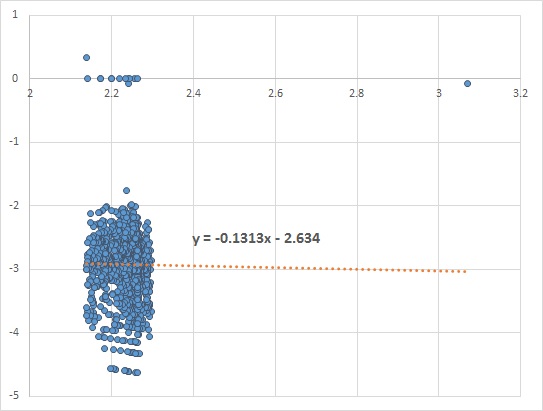

 , the yield
  equates the present value of the bond computed under a given set of rates. In other words:
 is a coupon paid out at time
  . Usually, one solves for
 be the price(or present value) of the bond expressed via its yield. Then, taking
  to represent interest rate, we have:
 and
and 
 where
where  our task is to estimate
  for
for  . Of course we may require to go outside of the range of our set of points, which would require extrapolation (or projection outside the known function values).
 and that
  . We can re-write this expression as follows:
 for
for  and
and  for
for  . Our linear interpolation is now taking a form of linear regression around
 ![[x_i, x_{i+1}]](https://s0.wp.com/latex.php?latex=%5Bx_i%2C+x_%7Bi%2B1%7D%5D&bg=ffffff&fg=111111&s=0&c=20201002) . The cubic spline can be defined as:
. The cubic spline can be defined as:
 and
and  coefficients, since
  . Take
  . The continuity condition (see P.R.Turner pg. 104) gives the following equalities:
 , we would be able to determine all the coefficients. After some re-arranging, it is possible to obtain:
 . This is a tridiagonal system of linear equations, which can be solved in a number of ways.
 . Using the above code we obtain the following results:

