A Tutorial on Hidden Markov Model with a Stock Price Example – Part 1

This tutorial is on a Hidden Markov Model. What is a Hidden Markov Model and why is it hiding?

I have split the tutorial in two parts. Part 1 will provide the background to the discrete HMMs. I will motivate the three main algorithms with an example of modeling stock price time-series. In part 2 I will demonstrate one way to implement the HMM and we will test the model by using it to predict the Yahoo stock price!

A Hidden Markov Model (HMM) is a statistical signal model. This short sentence is actually loaded with insight! A statistical model estimates parameters like mean and variance and class probability ratios from the data and uses these parameters to mimic what is going on in the data. A signal model is a model that attempts to describe some process that emits signals. Putting these two together we get a model that mimics a process by cooking-up some parametric form. Then we add “Markov”, which pretty much tells us to forget the distant past. And finally we add ‘hidden’, meaning that the source of the signal is never revealed. BTW, the later applies to many parametric models.

Setting up the Scene

HMM is trained on data that contains an observed sequence of signals (and optionally the corresponding states the signal generator was in when the signals were emitted). Once the HMM is trained, we can give it an unobserved signal sequence and ask:

How probable is that this sequence was emitted by this HMM? This would be useful for a problem like credit card fraud detection.
What is the most probable set of states the model was in when generating the sequence? This would be useful for a problem of time-series categorization and clustering.

It is remarkable that the model that can do so much was originally designed in the 1960-ies! Here we will discuss the 1-st order HMM, where only the current and the previous model states matter. Compare this, for example, with the nth-order HMM where the current and the previous n states are used. Here, by “matter” or “used” we will mean used in conditioning of states’ probabilities. For example, we will be asking about the probability of the HMM being in some state $q_{t}=s_{i}$ given that the previous state was $q_{t-1}=s_{j}$ . Such probabilities can be expressed in 2 dimensions as a state transition probability matrix. Let’s pick a concrete example. Let’s image that on the 4th of January 2016 we bought one share of Yahoo Inc. stock. Let’s say we paid $32.4 for the share. From then on we are monitoring the close-of-day price and calculating the profit and loss (PnL) that we could have realized if we sold the share on the day. The states of our PnL can be described qualitatively as being up, down or unchanged. Here being “up” means we would have generated a gain, while being down means losing money. The PnL states are observable and depend only on the stock price at the end of each new day. What generates this stock price? The stock price is generated by the market. The states of the market influence whether the price will go down or up. The states of the market can be inferred from the stock price, but are not directly observable. In other words they are hidden.

So far we have described the observed states of the stock price and the hidden states of the market. Let’s imagine for now that we have an oracle that tells us the probabilities of market state transitions. Generally the market can be described as being in bull or bear state. We will call these “buy” and “sell” states respectively. Table 1 shows that if the market is selling Yahoo stock, then there is a 70% chance that the market will continue to sell in the next time frame. We also see that if the market is in the buy state for Yahoo, there is a 42% chance that it will transition to selling next.

Table 1
	Sell	Buy
Sell	0.70	0.30
Buy	0.42	0.58

The oracle has also provided us with the stock price changes probabilities per market state. Table 2 shows that if the market is selling Yahoo, there is an 80% chance that the stock price will drop below our purchase price of $32.4 and will result in negative PnL. We also see that if the market is buying Yahoo, then there is a 10% chance that the resulting stock price will not be different from our purchase price and the PnL is zero. As I said, let’s not worry about where these probabilities come from. It will become clear later on. Note that row probabilities add to 1.0

Table 2
	Down	Up	Unchanged
Sell	0.80	0.15	0.05
Buy	0.25	0.65	0.10

It is February 10th 2016 and the Yahoo stock price closes at $27.1. If we were to sell the stock now we would have lost $5.3. Before becoming desperate we would like to know how probable it is that we are going to keep losing money for the next three days.

To put this in the HMM terminology, we would like to know the probability that the next three time-step sequence realised by the model will be {down, down, down} for t=1, 2, 3. This sequence of PnL states can be given a name $O=\{O_{1}, O_{2},O_{3}\}$ . So far the HMM model includes the market states transition probability matrix (Table 1) and the PnL observations probability matrix for each state (Table 2). Let’s call the former A and the latter B. We need one more thing to complete our HMM specification – the probability of stock market starting in either sell or buy state. Intuitively, it should be clear that the initial market state probabilities can be inferred from what is happening in Yahoo stock market on the day. But, for the sake of keeping this example more general we are going to assign the initial state probabilities as $\pi=\{0.5, 0.5\}$ . Thus we are treating each initial state as being equally likely. So, the market is selling and we are interested to find out $P(O|\lambda(A,B,\pi))$ . This is the probability to observe sequence $O$ given the current HMM parameterization. It is clear that sequence $O$ can occur under 2^3=8 different market state sequences. To solve the posed problem we need to take into account each state and all combinations of state transitions. The probability of this sequence being emitted by our HMM model is the sum over all possible state transitions and observing sequence values in each state.

Table 3
Sell, Sell, Sell
Sell, Sell, Buy
Sell, Buy, Sell
Sell, Buy, Buy
Buy, Sell, Sell
Buy, Buy, Sell
Buy, Sell, Buy
Buy, Buy, Buy

This gives rise to very long sum!

$P(O|\lambda)=P(\pi = sell)P(emit \, down \, from \, sell)P(move \, to \, sell \, from \, sell) \\ P(emit \, down \, from \, sell)P(move \, to \, sell \, from \, sell)P(emit \, down \, from \, sell) \\ + P(\pi = sell)P(emit \, down \, from \, sell)P(move \, to \, sell \, from \, sell)P(emit \, down \, from \, sell) \\ P(move \, to \, buy\, from \, sell)P(emit \, down \, from \, buy) \\ + ... \\ + P(\pi = buy)P(emit \, down \, from \, buy)P(move \, to \, sell \, from \, buy)P(emit \, down \, from \, sell) \\ P(move \, to \, sell \, from \, sell)P(emit \, down \, from \, sell) \\ + ... \\ + P(\pi = buy)P(emit \, down \, from \, buy)P(move \, to \, buy \, from \, buy)P(emit \, down \, from \, buy) \\ P(move \, to \, buy \, from \, buy)P(emit \, down \, from \, buy)$

In total we need to consider 2*3*8=48 multiplications (there are 6 in each sum component and there are 8 sums). That is a lot and it grows very quickly. Please note that emission probability is tied to a state and can be re-written as a conditional probability of emitting an observation while in the state. If we perform this long calculation we will get $P(O|\lambda=(A,B,\pi))=0.192$ . There is an almost 20% chance that the next three observations will be a PnL loss for us!

Oracle is No More

In the previous section we have gained some intuition about HMM parameters and some of the things the model can do for us. However, the model is hidden, so there is no access to oracle! The state and emission transition matrices we used to make projections must be learned from the data. The hidden nature of the model is inevitable, since in life we do not have access to the oracle. In life we have access to historical data/observations and a magic methods of “maximum likelihood estimation” (MLE) and Bayesian inference. The MLE essentially produces distributional parameters that maximize the probability of observing the data at hand (i.e. it gives you the parameters of the model that is most likely have had generated the data). The HMM has three parameters $\lambda=(A,B,\pi)$ . A fully specified HMM should be able to do the following:

Given a sequence of observed values, provide us with a probability that this sequence was generated by the specified HMM. This can be re-phrased as the probability of the sequence occurring given the model. This is what we have calculated in the previous section.
Given a sequence of observed values, provide us with the sequence of states the HMM most likely has been in to generate such values sequence.
Given a sequence of observed values we should be able to adjust/correct our model parameters $A$ , $B$ and $\pi$ .

When looking at the three ‘should’, we can see that there is a degree of circular dependency. That is, we need the model to do steps 1 and 2, and we need the parameters to form the model in step 3. Where do we begin? There are three main algorithms that are part of the HMM to perform the above tasks. These are: the forward&backward algorithm that helps with the 1st problem, the Viterbi algorithm that helps to solve the 2nd problem, and the Baum-Welch algorithm that puts it all together and helps to train the HMM model. Let’s discuss them next.

Going Back and Forth

That long sum we performed to calculate $P(O|\lambda=(A,B,\pi))$ grows exponentially in the number of states and observed values. The Forward and Backward algorithm is an optimization on the long sum. If you look back at the long sum, you should see that there are sum components that have the same sub-components in the product. For example,

$P(O|\lambda)=P(\pi = sell)P(emit \, down \, from \, sell)P(move \, to \, sell \, from \, sell)...$

appears twice. The HMM Forward and Backward (HMM FB) algorithm does not re-compute these, but stores the partial sums as a cache. There are $N$ states, $M$ discrete values that can be emitted from each of $s_{i,...,N}$ states and $i=1,...,N$ . There are $T$ observations in the considered sequence $O$ . The state transition matrix is $A$ , where $a_{i,j}$ is an individual entry and $j=1,...,N$ . The emission matrix is $B$ , where $b_{j}(O_{t})$ is an individual entry $b_{j}(T_{t})=P(emitting \, O_{t}|q_{t}=j)$ , and $t=1,...,T$ , $q_{t}$ is state at time t. For initial states we have $\pi_{i}=P(q_{1}=s_{i})$ . The problem of finding the probability of sequence $O$ given an HMM is $P(O|\lambda=(A,B,\pi))$ . Formally this probability can be expressed as a sum:

$P(O|\lambda)=\sum_{q_{1},q_{2},...,q_{T}}\pi_{q_{1}}b_{q_{1}}(O_{1})a_{q_{1}q_{2}}b_{q_{2}}(O_{2})a_{q_{2}q_{3}}b_{q_{3}}(O_{3})...a_{q_{T-1}q_{T}}b_{q_{T}}(O_{T})$

HMM FB calculates this sum efficiently by storing the partial sum calculated up to time $t$ . HMM FB is defined as follows:

Start by initializing the “cache” $\alpha_{1}(i)=\pi_{i}b_{i}(O_{1})$ , where $1 \le i \le N$ .
Calculate over all remaining observation sequences and states the partial sums:
$\alpha_{t+1}(j)=\big[\sum_{j=1}^{N} \alpha_{ij}\big] b_{j}(O_{t+1})$ , where $1 \le t \le T-1$ and $1 \le j \le N$ . Since at a single iteration we hold $i$ constant, this results in a trellis-like calculation along the columns of the transition matrix.
The probability is then given by $P(O|\lambda)=\sum_{i=1}^{N}\alpha_{T}(i)$ . This is where we gather the individual states probabilities together.

The above is the Forward algorithm which requires only $TN^{2}$ calculations. The algorithm moves forward. We can imagine an algorithm that performs similar calculation, but backwards, starting from the last observation in $O$ . Why do we need this? Is the Forward algorithm not enough? It is enough to solve the 1st poised problem. But it is not enough to solve the 3rd problem, as we will see later. So, let’s define the Backward algorithm now.

Start by initializing the end “cache” $\beta_{T}(i)=1$ , for $1 \le i \le N$ . This is an arbitrary assignment.
Calculate over all remaining observation sequences and states the partial sums (moving back to the start of the observation sequence):
$\beta_{t}(i)=\sum_{j=1}^{N} \alpha_{ij}b_{j}(O_{t+1})\beta_{t+1}(j)$ , where $t=T-1,T-2,...,1$ and $1 \le j \le N$ . Since at a single iteration we hold $i$ constant, this results in a trellis-like calculation along the columns of the transition matrix. However, it is performed backwards in time.

The $\beta$ matrix also contains probabilities of observing sequence $O$ . However, the actual values in $\beta$ are different from those in $\alpha$ because of the arbitrary assignment of $\beta_{T}$ to 1.

The State of the Affairs

We are now ready to solve the 2nd problem of the HMM – given the model and a sequence of observations, provide the sequence of states the model likely was in to generate such a sequence. Strictly speaking, we are after the optimal state sequence for the given $O$ . Optimal often means maximum of something. At each state and emission transitions there is a node that maximizes the probability of observing a value in a state. Let’s take a closer look at the $\alpha$ and $\beta$ matrices we calculated for the $\{down, \, down, \, down\}$ example.

I have circled the values that are maximum. All of these correspond to the Sell market state. Our HMM would have told us that the most likely market state sequence that produced $\{down, \, down, \, down\}$ was $\{Sell, \, Sell, \, Sell\}$ . Which makes sense. The HMM algorithm that solves the 2nd problem is called Viterbi Algorithm, named after its inventor Andrew Viterbi. The essence of Viterbi algorithm is what we have just done – find the path in the trellis that maximizes each node probability. It is a little bit more complex than just looking for the max, since we have to ensure that the path is valid (i.e. it is reachable in the specified HMM).

We are after the best state sequence $Q=\{q_{1},q_{2},...,q_{T}\}$ for the given $O$ . The best state sequence maximizes the probability of the path. We will be taking the maximum over probabilities and storing the indices of states that result in the max.

Start by initializing the end “cache” $\delta_{1}(j)=\pi_{i}b_{i}(O_{1})$ , for $1 \le i \le N$ . We also need to initialize to zero a variable used to track the index of the max node: $\phi_{1}(i)=0$ .
Calculate over all remaining observation sequences and states the partial max and store away the index that delivers it:
$\delta_{t}(j)=\max_{1\le i \le N} \small[ \delta_{t-1}(i)a_{ij}\small]b_{j}(O_{t})$ , where $2 \le t \le T$ and $1 \le j \le N$ .
Update the sequence of indices of the max nodes as:
$\phi_{t}=argmax_{1 \le i \le N} \small[ \delta_{t-1}(i) a_{ij}\small]$ for j and t as above.
Termination (probability and state):
$P*=\max_{1 \le i \le N} \small[\delta_{T}(i)\small]$
$q_{T}*=argmax_{1 \le i \le N} \small[\delta_{T}(i)\small]$
The optimal state sequence $Q$ is given by the path:
$q_{t}^{*}=\phi_{t+1}(q_{t+1}^{*})$ , for $t=T-1,T-2,...,1$

Expect the Unexpected

And now what is left is the most interesting part of the HMM – how do we estimate the model parameters from the data? We will now describe the Baum-Welch Algorithm to solve this 3rd poised problem.

The reason we introduced the Backward Algorithm is to be able to express a probability of being in some state i at time t and moving to a state j at time t+1. Imagine again the probabilities trellis. Pick a model state node at time t, use the partial sums for the probability of reaching this node, trace to some next node j at time t+1, and use all the possible state and observation paths after that until T. This gives the probability of being in state $s_{t}(i)$ and move to $s_{t+1}(j)$ . The figure below graphically illustrates this point.

To make this transition into a proper probability, we need to scale it by all possible transitions in $\lambda$ and $O$ . It can now be defined as follows:

$\gamma_{t}(i,j)=\frac{\alpha_{t}(i)a_{ij}b_{j}(O_{t+1})\beta_{t+1}(j)}{P(O|\lambda)}$

So, $\gamma_{t}(i,j)$ is a probability of being in state i at time t and moving to state j at time t+1. It makes perfect sense as long as we have true estimates for $\alpha$ , $A$ , $B$ and $\pi$ . We will come to these in a moment…

Summing $\gamma_{t}(i,j)$ across $j$ gives the probability of being in state i at time t under $O$ and $\lambda$ : $\gamma_{t}(i)=\sum_{j=1}^{N}\gamma_{t}(i,j)$ . Let’s look at an example to make things clear. Let’s consider $O=\{0,1,1\}=\{down, up, up\}$ . We will use the same $A$ and $B$ from Table 1 and Table 2. The $alpha$ learned for this observation sequence is shown below:

The (un-scaled) $\beta$ is shown below:

So, what is $\gamma_{1}(0,1)$ ? It is (0.7619*0.30*0.65*0.176)/0.05336=49%, where the denominator is calculated for $t=1$ . The denominator is calculated across all i and j at $t=1$ , thus it is a normalizing factor. If we calculate $\gamma_{2}(0,1)$ and sum the two estimates together, we will get the expected number of transitions from state $s(i)$ to $s(j)$ . Note, we do transition between two time-steps, but not from the final time-step as it is absorbing. Similarly, the sum over $\gamma_{t}(i)$ , where $t=1,2$ gives the expected number of transitions from $s(i)$ . It should now be easy to recognize that $\frac{\sum_{t=1}^{T-1}\gamma_{t}(i,j)}{\sum_{t=1}^{T-1}\gamma_{t}(i)}$ is the transition probability $a_{ij}$ , and this is how we estimate it:

$\hat{a_{ij}}=\frac{\sum_{t=1}^{T-1}\gamma_{t}(i,j)}{\sum_{t=1}^{T-1}\gamma_{t}(i)}$

We can derive the update to $b_{j}(O_{t})$ in a similar fashion. The matrix $B$ stores probabilities of observing a value from $O$ in some state. For $k=1,2,...,M$ $b_{j}(k)=\frac{\sum_{t\in\{1,...,T\}O_{t}=k}\gamma_{t}(j)}{\sum_{t=1}^{T}\gamma_{t}(j)}$ is the probability of observing symbol $k$ in state j. The update rule becomes:

$\hat{b_{j}}(k)=\frac{\sum_{t\in\{1,...,T\}O_{t}=k}\gamma_{t}(j)}{\sum_{t=1}^{T}\gamma_{t}(j)}$

$\pi$ stores the initial probabilities for each state. This parameter can be updated from the data as:

$\pi_{i}=\gamma_{1}(i)$

We now have the estimation/update rule for all parameters in $\lambda$ . The Baum-Welch algorithm is the following:

Repeat until convergence:
Initialize $A, B, \pi$ to random values such that $\pi_{i}\approx \frac{1}{N}$ , $a_{ij}\approx \frac{1}{N}$ and $b_{j}(k)\approx \frac{1}{M}$ . It is important to ensure that row probabilities add up to 1 and probabilities are not uniform as this may result in convergence to a local maximum.
Compute $\alpha_{t}(i)$ , $\beta_{t}(i)$ , and $\gamma_{t}(j)$ and $\gamma_{t}(i,j)$ .
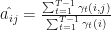
Re-estimate $A$ , $B$ , and $\pi$ .

The convergence can be assessed as the maximum change achieved in values of $A$ and $B$ between two iterations. The authors of this algorithm have proved that either the initial model defines the optimal point of the likelihood function and $\lambda = \hat{\lambda}$ , or the converged solution provides model parameters that are more likely for a given sequence of observations $O$ . The described algorithm is often called the expectation maximization algorithm and the observation sequence works like a pdf and is the “pooling” factor in the update of $\lambda$ . I have described the discrete version of HMM, however there are continuous models that estimate a density from which the observation come from, rather than a discrete time-series.

I hope some of you may find this tutorial revealing and insightful. I will share the implementation of this HMM with you next time.

Reference: L.R.Rabiner. An introduction to Hidden Markov models and selected applications in speech recognition. Proceedings of the IEEE, 77(2):257-268, 1989.