
Greetings, my blog readers!
In this post I would like to share with you two interesting visual insights into the effects of multicollinearity among the predictor variables on the coefficients of least squares regression (LSR). This post is very non-technical and I skip over most mathematical details. One of these insights is borrowed from Using Multivariate Statistics by Barbara Tabachnick and Linda Fidell (2013, 6th edition). When I first received it by post, after purchasing it on amazon, I immediately wanted to return it back. The paperback edition is the size of two large bricks and weighs 2.2 kg! I remember paging through it and thinking why on earth did this book receive so many good reviews on amazon. Only when I started reading it I understood why. This book is indispensable in providing clear and intuitive insight into topics like LSR, logistic regression, PCA and DA, canonical correlation, data cleaning and pre-processing, and many others. The source of the second insight is an online stats course offered by the Pennsylvania State University, which I find to be very good. Now that I am done with the credits, let’s see what the insights are!
I Thought you Said White with No Sugar?
Ok, so you probably know that multi/collinearity and singularity among predictor variables in regression is bad. But why is it bad and what does it affect? Multicollinearity is defined as a high (>90%) correlation among two or more predictor variables or their combinations (e.g. structural multicollinearity). Singularity can be simply defined as predictor redundancy. The presence of collinearity affects stability and interpretability of the regression model. By stability I mean what happens to the regression coefficients when new data points or new predictor variables are added in. By predictability I mean the usefulness of the magnitude and sign of the regression coefficients in telling the story. For example, economist are often interested in using regression models to explain the relationships of one set of economic parameters on another. Take for instance using inflation index and consumer price index to forecast borrow rates. The economists would be interested in building a model that can tell them that and x-amount increase in inflation will result in w*x-amount increase/decrease in the rate. Using predictor variables that are highly correlated with each other will most likely result in a model that “keeps changing” its story.
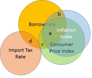
Let’s continue with our example of forecasting the borrow rate. Please note that in reality there may be no relationship between the borrow rate and inflation index or consumer price index. I am simply using these to illustrate the regression point. So, let’s imagine that inflation index (II) is correlated with the consumer price index (CPI) at 92%. Let’s also assume that we want to use the import tax rate (ITR) in the regression, as we believe that it is a factor in the inflation dynamics. Interestingly, ITR has no correlation with II and it correlates with CPI at 5%. We believe that the regression equation therefore is:

The LSR will estimate 

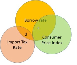
How does this make our regression solution unstable? Imagine we decide not to use II. The Venn diagram now looks like Figure 2. The regression coefficient of CPI will blow-up to the full credit it deserves. This will change our previous story about how CPI explains the borrow rate. If I were to remove the ITR instead, the coefficients of II and CPI would not have changed significantly. Thus in presence of multicollinearity among the predictor variables, neither do we get a stable solution, nor can we use it to properly interpret the underlying relationships.
Are you Sitting Comfortably?
Which chair would you rather sit on? Me too. In [2] we can find another great visual insight into how multicollinearity impacts the stability of LSR.

A scatter plot of two uncorrelated variables looks like a sea of data points. A scatter plot of two highly correlated variables looks more like a straight line. A regression solution will fit a hyperplane through the data points and the more spread-out the data points are, the more stable is the shape and direction of the best fit hyperplane. If, however, the data is align in a straight line, the best fit plane can be at any angle, depending on which target point it has to go through.

Figure 3 above shows that the uncorrelated data points act like anchors for the left hyperplane. In case of strongly correlated II and CPI where the data points are in a line, there are no anchors for the sides and corners of the right plane, and it will “tilt” into the direction of whichever BR point it has to go through.
Summary and Conclusion
I hope you have found this visual insight into the impact of multi/collinearity revealing. I definitely did. To conclude, the presence of multicollinearity among the predictor variables in the least squares standard multiple regression does not invalidate the predictions generated by the fitted model. However, the stability of the model and its usefulness in telling the story about the model parameters is compromised.
References:
[1]. Using Multivariate Statistics. Barbara Tabachnick and Linda Fidell. 2013, 6th edition. Pearson.
[2]. Online Statistics course STATS501. https://onlinecourses.science.psu.edu/stat501/
Notes:
(a) In practice, the total coefficients weight assigned to CPI and II will approximately reflect the entire a+b+c area. If CPI and II both have the same real contributions, the individual weights assigned by the regression may depend on the order of data columns (i.e. does CPI appear before II) that is used to fit regression model, with the first predictor receiving the greatest weight. By “lost to standard error” I mean the dependence on these random factors like order, as well as an overall increase in the standard error of CPI and II regression coefficients.
