On my blog space I am going to share with you example implementations of the most common machine learning techniques. The code will be either in C# or Python.
This is the first post in the series of several posts to come, which will be on algorithms commonly used to implement classifiers. A classifier is a machine learning algorithm that is allowed to build a representation of data on some training dataset, and ultimately is used to classify new unobserved instances. Classifiers are at the heart of machine learning and data mining, and they have wide use in medicine, speech and image recognition, and even finance. Broadly speaking all classifier fall into two categories: supervised and unsupervised. Supervised classifiers need to be ‘trained’, in the sense that they are fed the training data with known classifications, which is used to construct the priory. Unsupervised classifiers are a bit more complex, and work with unlabeled/unclassified training data (e.g. k-means clusters) or even have to learn the target class for each instance by trial and error (e.g. reinforced learning).
We’ll begin by looking at the most basic instance based classifier known as the K-Nearest Neighbour (kNN). Here K is the number of instances used to cast the vote when labeling previously unobserved instance. To demonstrate how kNN works, we will take this example dataset:
Table 1
| Attr 1 |
Attr 2 |
Attr 3 |
Class |
| 0.7 |
10 |
300 |
A |
| 0.14 |
9 |
120 |
A |
| 1.0 |
12 |
200 |
B |
| 1.12 |
15 |
300 |
B |
| 0.4 |
7 |
150 |
A |
| 0.6 |
8 |
600 |
A |
| 1.15 |
15 |
600 |
B |
| 1.12 |
11 |
400 |
B |
The above is a dataset with four columns and eight rows. The first three columns are the data (numerical format is required for kNN), the last column is the class. For the purpose of this example it does not matter what the data represents. I created random example with a hidden pattern, which, hopefully, our kNN algorithm can recognise.
Given previously unobserved instance I={i0,…,iN,class}, we calculate the Euclidean distance between I and each known instance in the dataset as follows:
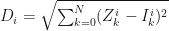
Here Z is a sequence of values of some instance i in attribute k for which a classification is given (see the dataset), and I is the unclassified instance.
For example, given I = {Attr1=12, Attr2=11, Attr3=500}, the resulting distance matrix, after normalisation, is the following:
Table 2
| D |
Class |
| 11.196 |
A |
| 11.772 |
A |
| 10.909 |
B |
| 10.792 |
B |
| 11.519 |
A |
| 11.295 |
A |
| 10.756 |
B |
| 10.774 |
B |
The distances were calculated on normalised data. That is, instead of using the original values in Table 1, where the 3rd column dominates all other values, we normalise each value according to:

Again, Z is from the dataset. The instance that we need to classify is also normalised. For example, the normalised values for Table 1 are:
Table 3
| Attr 1 |
Attr 2 |
Attr 3 |
Class |
| 0.554 |
0.375 |
0.375 |
A |
| 0 |
0.25 |
0 |
A |
| 0.851 |
0.625 |
0.167 |
B |
| 0.970 |
1 |
0.375 |
B |
| 0.257 |
0 |
0.062 |
A |
| 0.455 |
0.125 |
1 |
A |
| 1 |
1 |
1 |
B |
| 0.970 |
0.5 |
0.583 |
B |
The normalised I = {11.74, 0.5, 0.792}, which was calculated with max and min from the dataset, excluding the instance we need to classify.
Ok, now that we have calculated the distances (Table 2), we can proceed to vote on which class the instance I should belong to. To do this, we select K smallest distances and look at their corresponding classes. Let’s take K=3, then the smallest distances with votes are: 10.756 for B, 10.774 for B, and 10.792 for B. The new instance clearly belongs to class B. This is spot on, as the pattern is: Attr1<1 and Attr2<10 result in A, else B.
Consider another example I = {0.8, 11, 500}. For this instance, after normalisation, the top 3 distances with classes are: 0.379 for B, 0.446 for A, and 0.472 for A. The majority is A, so, the instance is classified as A.
Several modifications exist to the basic kNN algorithm. Some employ weights to improve classification, others use an even K and break ties in a weighted-fashion. Overall, it is a powerful, easy to implement classifier. If you are dealing with non-numeric data parameters, these can be quantified through some mapping from non-numeric value to numbers. Always remember to normalise your data, otherwise you are running a chance of introducing bias into the classifier.
Let’s now look at how kNN can be implemented with C#. At the start, I introduce several extensions to aid in data manipulation. In C#, extensions are an extremely useful concept and are quite addictive. And so is LINQ. You will notice that I try to use LINQ query where possible. Most worker method are private and my properties are read-only. Another thing to note is that my kNN constructor is private. Instead, the class users call initialiseKNN method which ensures that K is odd, since I am not using weights and don’t provide for tie breaks.
using System;
using System.Collections.Generic;
using System.Linq;
using System.Text;
using System.IO;

namespace kNN
{
    //extension method to aid in algorithm implementation
    public static class Extensions
    {
        //converts string representation of number to a double
        public static IEnumerable<double> ConvertToDouble<T>(this IEnumerable<T> array)
        {
            dynamic ds;
            foreach (object st in array)
            {
                ds = st;
                yield return Convert.ToDouble(ds);
            }
        }

        //returns a row in a 2D array
        public static T[] Row<T>(this T[,] array, int r)
        {
            T[] output = new T[array.GetLength(1)];
            if (r < array.GetLength(0))
            {
                for (int i = 0; i < array.GetLength(1); i++)
                    output[i] = array[r, i];
            }
            return output;
        }

        //converts a List of Lists to a 2D matrix
        public static T[,] ToMatrix<T>(this IEnumerable<List<T>> collection, int depth, int length)
        {
            T[,] output = new T[depth, length];
            int i = 0, j = 0;
            foreach (var list in collection)
            {
                foreach (var val in list)
                {
                    output[i, j] = val;
                    j++;
                }
                i++; j = 0;
            }

            return output;
        }

        //returns the classification that appears most frequently in the array of classifications
        public static string Majority<T>(this T[] array)
        {
            if (array.Length > 0)
            {
                int unique = array.Distinct().Count();
                if (unique == 1)
                    return array[0].ToString();

                return (from item in array
                             group item by item into g
                             orderby g.Count() descending
                             select g.Key).First().ToString();
            }
            else
                return "";
        }
    }

    /// <summary>
    /// kNN class implements the K Nearest Neighbor instance based classifier
    /// </summary>
    public sealed class kNN
    {
        //private constructor allows to ensure k is odd
        private  kNN(int K, string FileName, bool Normalise)
        {
            k = K;
            PopulateDataSetFromFile(FileName, Normalise);
        }

        /// <summary>
        /// Initialises the kNN class, the observations data set and the number of neighbors to use in voting when classifying
        /// </summary>
        /// <param name="K">integer representiong the number of neighbors to use in the classifying instances</param>
        /// <param name="FileName">string file name containing knows numeric observations with string classes</param>
        /// <param name="Normalise">boolean flag for normalising the data set</param>
        public static kNN initialiseKNN(int K, string FileName, bool Normalise)
        {
            if (K % 2 > 0)
                return new kNN(K, FileName, Normalise);
            else
            {
                Console.WriteLine("K must be odd.");
                return null;
            }
        }

        //read-only properties
        internal int K { get { return k; } }
        internal Dictionary<List<double>, string> DataSet { get { return dataSet;} }

        /// <summary>
        /// Classifies the instance according to a kNN algorithm
        /// calculates Eucledian distance between the instance and the know data
        /// </summary>
        /// <param name="instance">List of doubles representing the instance values</param>
        /// <returns>returns string - classification</returns>
        internal string Classify(List<double> instance)
        {
            int i=0;
            double [] normalisedInstance = new double[length];

            if (instance.Count!=length)
            {
                return "Wrong number of instance parameters.";
            }

            if (normalised)
            {
                foreach (var one in instance)
                {
                    normalisedInstance[i] = (one - originalStatsMin.ElementAt(i)) / (originalStatsMax.ElementAt(i) - originalStatsMin.ElementAt(i));
                    i++;
                }
            }
            else
            {
                normalisedInstance = instance.ToArray();
            }

            double[,] keyValue = dataSet.Keys.ToMatrix(depth, length);
            double[] distances = new double[depth];

            Dictionary<double, string> distDictionary = new Dictionary<double, string>();
            for (i = 0; i < depth; i++)
            {
                distances[i] = Math.Sqrt(keyValue.Row(i).Zip(normalisedInstance, (one, two) => (one - two) * (one - two)).ToArray().Sum());
                distDictionary.Add(distances[i], dataSet.Values.ToArray()[i]);

            }

            //select top votes
            var topK = (from d in distDictionary.Keys
                        orderby d ascending
                        select d).Take(k).ToArray();

            //obtain the corresponding classifications for the top votes
            var result = (from d in distDictionary
                        from t in topK
                        where d.Key==t
                        select d.Value).ToArray();

            return result.Majority();
        }
        /// <summary>
        /// Processess the file with the comma separated training data and populates the dictionary
        /// all values except for the class must be numeric
        /// the class is the last element in the dataset for each record
        /// </summary>
        /// <param name="fileName">string fileName - the name of the file with the training data</param>
        /// <param name="normalise">bool normalise - true if the data needs to be normalised, false otherwiese</param>
        private void PopulateDataSetFromFile(string fileName, bool normalise)
        {
            using (StreamReader sr = new StreamReader(fileName,true))
            {
                List<string> allItems = sr.ReadToEnd().TrimEnd().Split('\n').ToList();

                if (allItems.Count > 1)
                {
                    string[] array = allItems.ElementAt(0).Split(',');
                    length = array.Length - 1;
                    foreach (string item in allItems)
                    {
                        array = item.Split(',');
                        dataSet.Add(array.Where(p => p != array.Last()).ConvertToDouble().ToList(), array.Last().ToString().TrimEnd());
                    }
                    array = null;
                }
                else
                    Console.WriteLine("No items in the data set");
            }
            if (normalise)
            {
                NormaliseDataSet();
                normalised = true;
            }
        }

        private void NormaliseDataSet()
        {
            var keyCollection = from n in dataSet.Keys
                                select n;
            var valuesCollection = from n in dataSet.Values
                                   select n;

            depth = dataSet.Keys.Count;
            double[,] transpose = new double[length, depth];
            double[,] original = new double[depth, length];
            int i = 0, j = 0;

            //transpose
            foreach (var keyList in keyCollection)
            {
                foreach (var key in keyList)
                {
                    transpose[i, j] = key;
                    i++;
                }
                j++; i = 0;
            }

            //normalise
            double max, min;

            for (i = 0; i < length; i++)
            {
                originalStatsMax.Add (max = transpose.Row(i).Max());
                originalStatsMin.Add(min = transpose.Row(i).Min());

                for (j = 0; j < depth; j++)
                {
                    transpose[i, j] = (transpose[i, j] - min) / (max - min);
                }

            }
            for (i = 0; i < depth; i++)
            {
                for (j = 0; j < length; j++)
                    original[i, j] = transpose[j, i];
            }

            //overwrite the current values with the normalised ones
            dataSet = new Dictionary<List<double>, string>();
            for (i = 0; i < depth; i++)
            {
                dataSet.Add(original.Row(i).ToList(), valuesCollection.ElementAt(i));
            }
        }

        //private members
        private Dictionary<List<double>, string> dataSet = new Dictionary<List<double>,string>();
        private List<double> originalStatsMin = new List<double>();
        private List<double> originalStatsMax = new List<double>();
        private int k=0;
        private int length=0;
        private int depth=0;
        private bool normalised = false;
    }

    class EntryPoint
    {
        static void Main(string[] args)
        {
            kNN examplekNN = kNN.initialiseKNN(3,"DataSet.txt",true);

            List<double> instance2Classify = new List<double> {12,11,500};
            string result = examplekNN.Classify(instance2Classify);
            Console.WriteLine("This instance is classified as: {0}", result);
            Console.ReadLine();
        }
    }
}
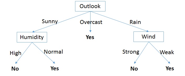
In my next blog we will look at decision trees – a slightly more complicated, but also more powerful machine learning algorithm.


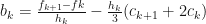
 where
where  our task is to estimate
  for
for  . Of course we may require to go outside of the range of our set of points, which would require extrapolation (or projection outside the known function values).
 and that
  . We can re-write this expression as follows:
 for
for  and
and  for
for  . Our linear interpolation is now taking a form of linear regression around
 ![[x_i, x_{i+1}]](https://s0.wp.com/latex.php?latex=%5Bx_i%2C+x_%7Bi%2B1%7D%5D&bg=ffffff&fg=111111&s=0&c=20201002) . The cubic spline can be defined as:
. The cubic spline can be defined as:
 and
and  coefficients, since
  . Take
  . The continuity condition (see P.R.Turner pg. 104) gives the following equalities:
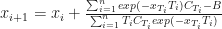
 , we would be able to determine all the coefficients. After some re-arranging, it is possible to obtain:
 . This is a tridiagonal system of linear equations, which can be solved in a number of ways.
 . Using the above code we obtain the following results:


 is logarithm base 2. The base two is due to the entropy being a measure of the expected encoding in binary format (i.e. 0s and 1s). Note that the smaller are individual probabilities, the greater is the absolute value of entropy. Also, the closer is entropy to zero, the more order there is in the data.
 , accurate to 3 d.p. There is a reason why we started with the class column. It will be used to measure the information gain we can achieve by splitting the data one attribute/column at a time, which is the core idea behind building decision trees. At each step we will be picking the attribute that achieves the greatest information gain to split the tree recursively. The information gain is, essentially, a positive difference in entropy; and the root node of any decision tree is the attribute with the greatest information gain. Information gain is formally defined as:
 and
and  are the number of records taking on the value i and the total number of records respectively. Finally,
  is the corresponding entropy of all records where the attribute A takes on value i with respect to the target class. The last sentence is important. It means that, given all the records where attribute A takes on the same value i we are interested to know the dispersion of the target class. For example, take a look at all the records where Wind is strong. Here we have 3 records where the target class is ‘no’ and 3 records where it is ‘yes’. Thus, the corresponding entropy is


 .
.

![X=F^{-1} (U),U\approx Unif[0,1]](https://s0.wp.com/latex.php?latex=X%3DF%5E%7B-1%7D+%28U%29%2CU%5Capprox+Unif%5B0%2C1%5D&bg=ffffff&fg=111111&s=0&c=20201002)
 is the inverse of the cumulative distribution function (i.e. any given c.d.f.), and X is the desired random variable satisfying
  property. Again, the c.d.f. can be for any required distribution for which the inverse is well-defined.
 . Figure 1 shows the probability on the y-axis and the random variable on the x-axis. The probability axis corresponds to the uniform random variable range, which is [0,1]. Thus, we can use the y-axis to map to the x-axis, which would give us a random variable in (-3,3) interval. This random variable is normally distributed with mean 0 and standard deviation of 1. In Figure 1 I have marked the middle of both axis to make it clear that uniform random variables between 0 and 0.5 would map to normal random variables that are negative. The uniforms above 0.5 map to positive r.vs.


 and
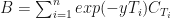
and  are constants (see the code for their values). The above is defined for
  . For
. For  , we can utilize Chebyshev’s approximation, as demonstrated in [1]:
 over the [-7,7] range for x.


 , such that
  follows exponential distribution with mean 2 and
  (i.e. bivariate normal).
