
To continue my blogging on machine learning (ML) classifiers, I am turning to decision trees. The post on decision trees will be in two parts. Part 1 will provide an introduction to how decision trees work and how they are build. Part 2 will contain the C# implementation of an example decision trees classifier. As in all my posts, I prefer clear and informal explanation over the terse mathematical one. So, any pedants out there – look away now!
Decision trees are a great choice for inductive inference and have been widely used for a long time in the field of Artificial Intelligence (AI). In this post we will cover the decision tree algorithm known as ID3.
There are several reasons why decision trees are great classifiers:
- decision trees are easy to understand;
- decision trees work well with messy data or missing values;
- decision trees give insight into complex data;
- decision trees can be visualized to allow for inference inspection or correction;
- decision tree building algorithms can be as simple or sophisticated as required (e.g. they can incorporate pruning, weights, etc.);
Decision trees work best with discrete classes. That is, the output class for each instance is either a string, boolean or an integer. If you are working with continuous values, you may consider rounding and mapping to a discrete output class, or may need to look for another classifier. Decision trees are used for classification problems. For example, the taxonomy of organisms, plants, minerals, etc. lends itself naturally to decision tree classifiers. This is because in a field of taxonomy we are dealing with a set of records containing values for some attributes. The values come from a finite set of known features. Each record may or may not have a classification. Medicine is another field that makes use of decision trees. Almost all illnesses can be categorized by symptoms, thus decision trees aid doctors in illness diagnosis.
It is time for an example, which I am borrowing from [1]. The tennis playing example in ML is like the ‘Hello World’ in programming languages. We are given some data about the weather conditions that are appropriate for playing tennis. Our task is to construct a decision tree based on this data, and use the tree to classify unknown weather conditions. The learning data is:
| Outlook | Temperature | Humidity | Wind | Play Tennis |
|---|---|---|---|---|
| sunny | hot | high | strong | no |
| sunny | hot | high | weak | no |
| overcast | hot | high | weak | yes |
| rain | mild | high | weak | yes |
| rain | cool | normal | weak | yes |
| rain | cool | normal | strong | no |
| overcast | cool | normal | strong | yes |
| sunny | mild | high | weak | no |
| sunny | cool | normal | weak | yes |
| rain | mild | normal | weak | yes |
| sunny | mild | normal | strong | yes |
| overcast | mild | high | strong | yes |
| overcast | hot | normal | weak | yes |
| rain | mild | high | strong | no |
Table 1 tells us which weather conditions are good for playing tennis outdoors. For example, if it is sunny, and the wind is weak, and the temperature is mild but it is very humid, then playing tennis outdoors is not advisable. On the other hand, on an overcast day, regardless of the wind, playing tennis outdoors should be OK.
The most fundamental concept behind the decision tree classifiers is that of order. The amount of order in the data can be measured by assessing its consistency. For example, imagine that every row in Table 1 had a ‘yes’ associated with the Play Tennis column. This would tell us that regardless of the wind, temperature, humidity, we can always play tennis outside. The data would have perfect order, and we would be able to build a perfect classifier for the data – the one that always says ‘yes’ and is always correct. The other extreme would be where the outcome class differs for every observation. For an inductive learner like a decision tree, this would mean that it is impossible to classify new instance unless it perfectly matches some instance in the training set. This is why decision tree classifier won’t work for continuous class problems.
In information theory the concept of order (actually, lack of it), is often represented by entropy. It is a scary word for something that is rather simple. Entropy definition was proposed by the founder of information theory – Claude Shannon, and it is a probabilistic measure of categorical data defined as:

where S is the training data set with some target classification that takes on n different values. The discrete target values are assigned their probabilities p, and 
We now can calculate the entropy of our data, one column at a time. Let’s take the Play Tennis column. We have 9 ‘yes’ and 5 ‘no’, this gives us the entropy of 

where A is the set of all values some attribute takes. For example, the Wind column takes values in {strong, weak}, and the Humidity column takes on values in {high, normal}. 


So, which attribute/column should be the tree’s root node? It should be the one that achieves the greatest information gain:


It is clear that Outlook achieves the greatest information gain and should be the root of the tree. The worst information gain would be achieved with Temperature attribute. This is what our tree now looks:

At this stage we have the training data split into three clusters. Where outlook is overcast, we have a target class of ‘yes’. We now proceed recursively building the sub-tree in the other two clusters. Where outlook is sunny, we have a total of 5 records. These are reproduced in Table 2 below. Out of three possible attributes for the node we again pick the one that achieves the greatest information gain. If you inspect the data in Table 2, it is easy to see that humidity is that attribute since all five records can be split as following: if humidity is normal, then ‘yes’, else ‘no’. Its corresponding information gain is

where 0.970 is entropy of Outlook is sunny, again, with respect to the Play Tennis class:
| Outlook | Temperature | Humidity | Wind | Play Tennis |
|---|---|---|---|---|
| sunny | hot | high | strong | no |
| sunny | hot | high | weak | no |
| sunny | mild | high | weak | no |
| sunny | cool | normal | weak | yes |
| sunny | mild | normal | strong | yes |
At this stage we have classified 9 records and our tree has 9 terminal descendant nodes (leaves):

We can now deal with the records in the last outlook cluster, i.e. where outlook is rain. Here we have five records, which are reproduced below in Table 3:
| Outlook | Temperature | Humidity | Wind | Play Tennis |
|---|---|---|---|---|
| rain | mild | high | weak | yes |
| rain | cool | normal | weak | yes |
| rain | cool | normal | strong | no |
| rain | mild | normal | weak | yes |
| rain | mild | high | strong | no |
We apply the same algorithm as before by selecting the attribute for the next node that gives the greatest information gain. It is easy to spot that the Wind attribute achieves just that. Its total information gain is

The complete tree looks like this:
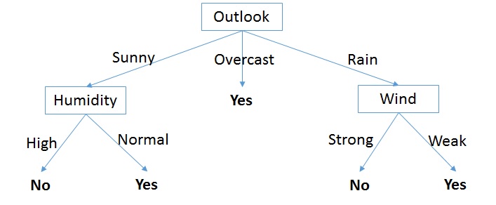
A few things should be noted about the final decision tree. Firstly, the Temperature attribute is completely missing. The constructed decision tree allowed us to see that this attribute is redundant, at least given the training dataset. Decision trees always favor the shorter trees over the longer ones, which is the main part of its inductive bias (or the algorithm’s policy). Secondly, this is not a binary tree, since we have parent nodes with more than two edges (i.e. the Outlook node). Finally, the constructed decision tree allows for a one-way searching algorithm. This means that we cannot back-track to the parent node. In the grand scheme of things this implies that a decision tree can end up at a locally optimal, rather than globally optimal solution.
The next blog post will be on how to implement the decision tree classifier in C#.
References:
[1]. T.M.Mitchell. Machine Learning. McGraw-Hill. 1997.
