Absolute vs. Proportional Returns

Greetings, my blog readers!

It will be a safe assumption to make that people who read my blogs work with data. In finance, the data is often in form of asset prices or other market indicators like implied volatility. Analyzing price data often requires calculating returns (aka. moves). Very often we work with proportional returns or log returns. Proportional returns are calculated relative to the price level. For example, given any two historical prices x_{t} and x_{t+h}, the proportional change is:

m_{t,prop} = \frac{x_{t+h}-x_{t}}{x_t}

The above can be shortened as m_{t, prop} = \frac{x_{t+h}}{x_t}-1. In contrast, absolute moves are defined simply as the difference between two historical price observations: m_{t,abs} = x_{t+h}-x_{t}.

How do you know which type of return is appropriate for your data? The answer depends on the price dynamic and the simulation/analysis task at hand. Historical simulation, often used in Value-at-Risk (VaR), requires calculating PnL strip from some sensitivity and a set of historical returns. For example, a VaR model for foreign exchange options may be specified to take into account PnL impact from changes in implied volatility skew. Here, the PnL is historically simulated using sensitivities of a volatility curve or surface and historical implied volatility returns for some surface parameter, like low risk reversal. You have a choice in how to calculate the volatility returns. The right choice can be determined with a simple regression.

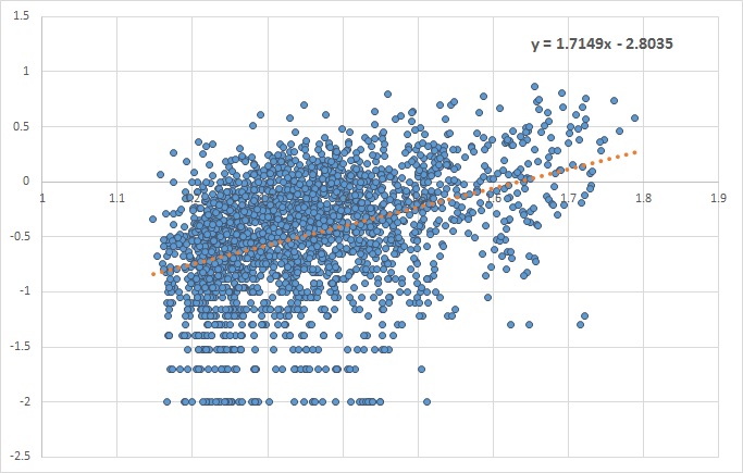
Essentially, we need to look for evidence of dependency of price returns on price levels. In FX, liquid options on G21 currency pairs do not exhibit such dependency, while emerging market pairs do. I have not been able to locate a free source of implied FX volatility, but I have found two instruments that are good enough to demonstrate the concept. CBOE LOVOL Index is a low volatility index and can be downloaded for free from Quandl. For this example I took the close of day prices from 2012-2017. After plotting log_{10}(ABS(x_{t})) vs. log_{10}(ABS(m_{t,abs})) we look for the value of the slope of the fitted linear line. A slope closer to zero indicates no dependency, while a positive or negative slope shows that the two variables are dependent.

CBOE LVOL

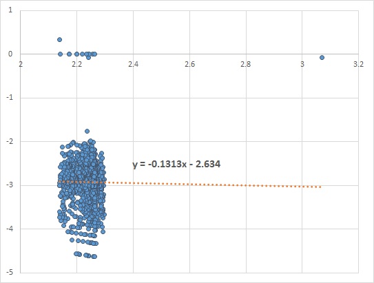
In the absence of dependency, absolute returns can be used, while proportional return are otherwise more appropriate. Take a look at a plot of VXMT CBOE Mid-term Volatility Index. The fitted linear line has a slope of approximately 1.7. Historical simulation of VXMT is calling for proportional rather than absolute price moves.

CBOE VXMT

Hidden Technical Debt of Machine Learning – Play Now Pay Later

Last week I was lucky enough to attend the Strata Conference London 2017 for one day. The venue and the event are impressive in scale, participants and content. The quality of tutorials and talks, in general, was very good, and I have walked away with a few new ideas I wanted to share on my blog.

One of the most important lessons from the conference for me was from a reference to the NIPS’16 paper titled Hidden Technical Debt in Machine Learning System, written by Google researchers. The paper is about the long-term maintenance costs introduced by building machine learning (ML) models and systems. The argument is that such cost is hidden as it is not immediately apparent from the point of putting an ML model in production. For data scientists it is important to be aware of the complexity of the models they develop and what impact these models will have on their organisation and how much it will cost to maintain them.

According to the authors, there are three levels of technical complexity which contribute to technical debt in ML: the model itself can be complex and behave non-linearly to a given set of parameters, the model can be taking input from otherwise disparate systems, and the model’s output or its behavior can be complex and difficult to predict before it is released.

ML Model Complexity

ML models entangle input signals from different systems together, making it difficult to avoid the CACE principle: Change Anything Change Everything. This principle applies to all aspects of ML, from parameters (think xgboost!), to input data to convergence thresholds and sampling methods. Isolation and servicing of modelling components is one of the proposed solutions.

The Cost  of Data Dependencies

Large ML systems have large and complex data dependencies, where data quality and any data assumptions can significantly affect the ML system output. ML system input data can be unstable, meaning it changes qualitatively and quantitatively over time. In some cases, the degree of dependency on one set of data vs. another may change. The ML systems are unique because usually their data dependencies are finer (e.g. the input should not just be an integer, but an integer in a certain range). A lot of thinking and possibly investment should go into understanding such dependencies and controlling them. Check-out kensu.io – a start-up company I have come across at the conference, the creators of Adalog – a product designed purely for such task.

The Feedback Loop and Dealing with Changes

Live ML systems learn in real time and influence their own behavior. Sometimes it is necessary to choose static parameters, like prediction thresholds, for a model that is trained or parameterised on  data that is dynamic in nature. Thus leading to the previous set of thresholds being no longer valid on updated data. The authors highlight that comprehensive monitoring of ML system behavior is critical for long-term system reliability.

In summary, maintainable ML systems are costly and require an even higher level of technical competence and foresight among its developers.  ML models testing, validation and monitoring should be considered as an absolute must in organisations that are eager to rip their full benefits.

(Jan-17) Did You Know That?

A brand new idea for my blog in 2017 is a monthly Did You Know That digest where I am going to share with you m things (where m<=3) that I recently learnt and found to be useful. I am going to keep such digests short and simple, as not to overwhelm you with verbiage and unnecessary details. This month’s top 3 Did you know that? are:

  • scikit-learn SGDClassifier – one learner, many tricks up its sleeve;
  • GraphViz is integrated in scikit-learn – no need no import it separately!
  • Zeppelin notebook from Apache – worth a look if you are into Python notebooks;

scikit-learn SGDClassifier

This is a multi-classifier module that implements stochastic gradient descent. The loss parameter controls which model is used to train and perform classification. For example, loss=hinge will give a linear SVM, and loss=log will give a logistic regression. When should you use it? When your training data set does not fit into memory. Note that SGD also allows mini-batch learning.

GraphViz is Integrated in scikit-learn Decision Trees

If you read all my blog post, you may have come across this one where I put together some code to train a binary decision tree to recognize a hand in poker. The code is available on my github space. If you read the code, you will see that I defined graph_decision_tree method with all the hula-loops to graph and save the images. But did you know that you don’t need to do all this work since sklearn.tree has export_graphviz module? If dsTree is an instance of DecisionTreeClassifier, then one can simply do:

from sklearn.tree import export_graphviz

export_graphviz(dsTree, out_file='dsTree.dot',
       feature_names=['feature1', 'feature2'])

The .dot file can be converted to a .png file (if you have installed GraphViz) like this:

dot -Tpng tree.dot -o tree.png

Zeppelin Notebook from Apache

If you are using Apache Spark you may be glad to learn that Apache has a notebook to go along with it. Zeppelin notebook offers similar functionality to Jupyter in terms of data visualization, paragraph writing and notebook sharing. I recommend that you to check it out.