This is the 2nd part of the tutorial on Hidden Markov models. In this post we will look at a possible implementation of the described algorithms and estimate model performance on Yahoo stock price time-series.
Implementation of HMM in Python
I am providing an example implementation on my GitHub space. Please note that all code is provided with a disclaimer that you are free to use it at your own risk. HMM.py contains the main implementation. There are a few things to point out in this file:
As is pointed out in the referenced document in part 1, and require to be scaled for longer observations since the product of probabilities quickly tends to zero, resulting in underflow. The code has a flag for scaling, and defaults to positive.
While testing out this model I noticed that initial assignment of and makes a big difference to the final solution. I am providing two possible assignments. One, as described in part 1, setting approximately to the same values, adding to 1. And two, using Dirichlet distribution to create non-uniform assignment that adds-up to 1. I’ve noticed that the former results in more meaningful model parameters.
You will notice a small hack in HMMBaumWelch method where I am setting to the maximum observation in . This is needed because not all observation sequences will contain all values (i.e. 0, 1, 2). And the transition and emission matrices are accessed as if all the values exist.
I am using yahoo_finance Python module to source the stock prices for Yahoo. It seems to work and is pretty easy to use. You should be able to download this module here.
HMM Model performance to predict Yahoo stock price move
On my github space, HMM_test.py contains a possible test example code. I am testing the model as following: train the model on a specified window of daily historical moves (e.g. 10 days) and using the model parameters determine the predicted current model state. Then, using the predicted state, determine the next likely state from :
prediction_state = np.argmax(a[path[-1],:])
The most likely emitted value from that state can be found as follows:
prediction = np.argmax(b[prediction_state,:])
I then compare the predicted move to the historical one. So, how did HMM do? Well, not so well. The model parameters are very sensitive to the convergence tolerance, initial assignment and, obviously the training time-window. Calculating accuracy ratio as the number of correctly predicted directions is pretty much around 50%-56% (tests on more recent data produce the higher accuracy in this range). Thus, we might as well be throwing a coin to make buy or sell predictions. It is possible that EOD price moves are not granular enough to provide a coherent market dynamic model.
This tutorial is on a Hidden Markov Model. What is a Hidden Markov Model and why is it hiding?
Can you see me?
I have split the tutorial in two parts. Part 1 will provide the background to the discrete HMMs. I will motivate the three main algorithms with an example of modeling stock price time-series. In part 2 I will demonstrate one way to implement the HMM and we will test the model by using it to predict the Yahoo stock price!
A Hidden Markov Model (HMM) is a statistical signal model. This short sentence is actually loaded with insight! A statistical model estimates parameters like mean and variance and class probability ratios from the data and uses these parameters to mimic what is going on in the data. A signal model is a model that attempts to describe some process that emits signals. Putting these two together we get a model that mimics a process by cooking-up some parametric form. Then we add “Markov”, which pretty much tells us to forget the distant past. And finally we add ‘hidden’, meaning that the source of the signal is never revealed. BTW, the later applies to many parametric models.
Setting up the Scene
HMM is trained on data that contains an observed sequence of signals (and optionally the corresponding states the signal generator was in when the signals were emitted). Once the HMM is trained, we can give it an unobserved signal sequence and ask:
How probable is that this sequence was emitted by this HMM? This would be useful for a problem like credit card fraud detection.
What is the most probable set of states the model was in when generating the sequence? This would be useful for a problem of time-series categorization and clustering.
It is remarkable that the model that can do so much was originally designed in the 1960-ies! Here we will discuss the 1-st order HMM, where only the current and the previous model states matter. Compare this, for example, with the nth-order HMM where the current and the previous n states are used. Here, by “matter” or “used” we will mean used in conditioning of states’ probabilities. For example, we will be asking about the probability of the HMM being in some state given that the previous state was . Such probabilities can be expressed in 2 dimensions as a state transition probability matrix. Let’s pick a concrete example. Let’s image that on the 4th of January 2016 we bought one share of Yahoo Inc. stock. Let’s say we paid $32.4 for the share. From then on we are monitoring the close-of-day price and calculating the profit and loss (PnL) that we could have realized if we sold the share on the day. The states of our PnL can be described qualitatively as being up, down or unchanged. Here being “up” means we would have generated a gain, while being down means losing money. The PnL states are observable and depend only on the stock price at the end of each new day. What generates this stock price? The stock price is generated by the market. The states of the market influence whether the price will go down or up. The states of the market can be inferred from the stock price, but are not directly observable. In other words they are hidden.
So far we have described the observed states of the stock price and the hidden states of the market. Let’s imagine for now that we have an oracle that tells us the probabilities of market state transitions. Generally the market can be described as being in bull or bear state. We will call these “buy” and “sell” states respectively. Table 1 shows that if the market is selling Yahoo stock, then there is a 70% chance that the market will continue to sell in the next time frame. We also see that if the market is in the buy state for Yahoo, there is a 42% chance that it will transition to selling next.
Table 1
Sell
Buy
Sell
0.70
0.30
Buy
0.42
0.58
The oracle has also provided us with the stock price changes probabilities per market state. Table 2 shows that if the market is selling Yahoo, there is an 80% chance that the stock price will drop below our purchase price of $32.4 and will result in negative PnL. We also see that if the market is buying Yahoo, then there is a 10% chance that the resulting stock price will not be different from our purchase price and the PnL is zero. As I said, let’s not worry about where these probabilities come from. It will become clear later on. Note that row probabilities add to 1.0
Table 2
Down
Up
Unchanged
Sell
0.80
0.15
0.05
Buy
0.25
0.65
0.10
It is February 10th 2016 and the Yahoo stock price closes at $27.1. If we were to sell the stock now we would have lost $5.3. Before becoming desperate we would like to know how probable it is that we are going to keep losing money for the next three days.
To put this in the HMM terminology, we would like to know the probability that the next three time-step sequence realised by the model will be {down, down, down} for t=1, 2, 3. This sequence of PnL states can be given a name . So far the HMM model includes the market states transition probability matrix (Table 1) and the PnL observations probability matrix for each state (Table 2). Let’s call the former A and the latter B. We need one more thing to complete our HMM specification – the probability of stock market starting in either sell or buy state. Intuitively, it should be clear that the initial market state probabilities can be inferred from what is happening in Yahoo stock market on the day. But, for the sake of keeping this example more general we are going to assign the initial state probabilities as . Thus we are treating each initial state as being equally likely. So, the market is selling and we are interested to find out . This is the probability to observe sequence given the current HMM parameterization. It is clear that sequence can occur under 2^3=8 different market state sequences. To solve the posed problem we need to take into account each state and all combinations of state transitions. The probability of this sequence being emitted by our HMM model is the sum over all possible state transitions and observing sequence values in each state.
Table 3
Sell, Sell, Sell
Sell, Sell, Buy
Sell, Buy, Sell
Sell, Buy, Buy
Buy, Sell, Sell
Buy, Buy, Sell
Buy, Sell, Buy
Buy, Buy, Buy
This gives rise to very long sum!
In total we need to consider 2*3*8=48 multiplications (there are 6 in each sum component and there are 8 sums). That is a lot and it grows very quickly. Please note that emission probability is tied to a state and can be re-written as a conditional probability of emitting an observation while in the state. If we perform this long calculation we will get . There is an almost 20% chance that the next three observations will be a PnL loss for us!
Oracle is No More
Neo Absorbs Fail
In the previous section we have gained some intuition about HMM parameters and some of the things the model can do for us. However, the model is hidden, so there is no access to oracle! The state and emission transition matrices we used to make projections must be learned from the data. The hidden nature of the model is inevitable, since in life we do not have access to the oracle. In life we have access to historical data/observations and a magic methods of “maximum likelihood estimation” (MLE) and Bayesian inference. The MLE essentially produces distributional parameters that maximize the probability of observing the data at hand (i.e. it gives you the parameters of the model that is most likely have had generated the data). The HMM has three parameters . A fully specified HMM should be able to do the following:
Given a sequence of observed values, provide us with a probability that this sequence was generated by the specified HMM. This can be re-phrased as the probability of the sequence occurring given the model. This is what we have calculated in the previous section.
Given a sequence of observed values, provide us with the sequence of states the HMM most likely has been in to generate such values sequence.
Given a sequence of observed values we should be able to adjust/correct our model parameters , and .
When looking at the three ‘should’, we can see that there is a degree of circular dependency. That is, we need the model to do steps 1 and 2, and we need the parameters to form the model in step 3. Where do we begin? There are three main algorithms that are part of the HMM to perform the above tasks. These are: the forward&backward algorithm that helps with the 1st problem, the Viterbi algorithm that helps to solve the 2nd problem, and the Baum-Welch algorithm that puts it all together and helps to train the HMM model. Let’s discuss them next.
Going Back and Forth
That long sum we performed to calculate grows exponentially in the number of states and observed values. The Forward and Backward algorithm is an optimization on the long sum. If you look back at the long sum, you should see that there are sum components that have the same sub-components in the product. For example,
appears twice. The HMM Forward and Backward (HMM FB) algorithm does not re-compute these, but stores the partial sums as a cache. There are states, discrete values that can be emitted from each of states and . There are observations in the considered sequence . The state transition matrix is , where is an individual entry and . The emission matrix is , where is an individual entry , and , is state at time t. For initial states we have . The problem of finding the probability of sequence given an HMM is . Formally this probability can be expressed as a sum:
HMM FB calculates this sum efficiently by storing the partial sum calculated up to time . HMM FB is defined as follows:
Start by initializing the “cache” , where .
Calculate over all remaining observation sequences and states the partial sums: , where and . Since at a single iteration we hold constant, this results in a trellis-like calculation along the columns of the transition matrix.
The probability is then given by . This is where we gather the individual states probabilities together.
The above is the Forward algorithm which requires only calculations. The algorithm moves forward. We can imagine an algorithm that performs similar calculation, but backwards, starting from the last observation in . Why do we need this? Is the Forward algorithm not enough? It is enough to solve the 1st poised problem. But it is not enough to solve the 3rd problem, as we will see later. So, let’s define the Backward algorithm now.
Start by initializing the end “cache” , for . This is an arbitrary assignment.
Calculate over all remaining observation sequences and states the partial sums (moving back to the start of the observation sequence): , where and . Since at a single iteration we hold constant, this results in a trellis-like calculation along the columns of the transition matrix. However, it is performed backwards in time.
The matrix also contains probabilities of observing sequence . However, the actual values in are different from those in because of the arbitrary assignment of to 1.
The State of the Affairs
We are now ready to solve the 2nd problem of the HMM – given the model and a sequence of observations, provide the sequence of states the model likely was in to generate such a sequence. Strictly speaking, we are after the optimal state sequence for the given . Optimal often means maximum of something. At each state and emission transitions there is a node that maximizes the probability of observing a value in a state. Let’s take a closer look at the and matrices we calculated for the example.
Example Alpha and Beta
I have circled the values that are maximum. All of these correspond to the Sell market state. Our HMM would have told us that the most likely market state sequence that produced was . Which makes sense. The HMM algorithm that solves the 2nd problem is called Viterbi Algorithm, named after its inventor Andrew Viterbi. The essence of Viterbi algorithm is what we have just done – find the path in the trellis that maximizes each node probability. It is a little bit more complex than just looking for the max, since we have to ensure that the path is valid (i.e. it is reachable in the specified HMM).
We are after the best state sequence for the given . The best state sequence maximizes the probability of the path. We will be taking the maximum over probabilities and storing the indices of states that result in the max.
Start by initializing the end “cache” , for . We also need to initialize to zero a variable used to track the index of the max node: .
Calculate over all remaining observation sequences and states the partial max and store away the index that delivers it: , where and .
Update the sequence of indices of the max nodes as: for j and t as above.
Termination (probability and state):
The optimal state sequence is given by the path: , for
Expect the Unexpected
And now what is left is the most interesting part of the HMM – how do we estimate the model parameters from the data? We will now describe the Baum-Welch Algorithm to solve this 3rd poised problem.
The reason we introduced the Backward Algorithm is to be able to express a probability of being in some state i at time t and moving to a state j at time t+1. Imagine again the probabilities trellis. Pick a model state node at time t, use the partial sums for the probability of reaching this node, trace to some next node j at time t+1, and use all the possible state and observation paths after that until T. This gives the probability of being in state and move to . The figure below graphically illustrates this point.
Starting in i and moving to j.
To make this transition into a proper probability, we need to scale it by all possible transitions in and . It can now be defined as follows:
So, is a probability of being in state i at time t and moving to state j at time t+1. It makes perfect sense as long as we have true estimates for , , and . We will come to these in a moment…
Summing across gives the probability of being in state i at time t under and : . Let’s look at an example to make things clear. Let’s consider . We will use the same and from Table 1 and Table 2. The learned for this observation sequence is shown below:
Alpha for O={0,1,1}
The (un-scaled) is shown below:
Beta for O={0,1,1}
So, what is ? It is (0.7619*0.30*0.65*0.176)/0.05336=49%, where the denominator is calculated for . The denominator is calculated across all i and j at , thus it is a normalizing factor. If we calculate and sum the two estimates together, we will get the expected number of transitions from state to . Note, we do transition between two time-steps, but not from the final time-step as it is absorbing. Similarly, the sum over , where gives the expected number of transitions from . It should now be easy to recognize that is the transition probability , and this is how we estimate it:
We can derive the update to in a similar fashion. The matrix stores probabilities of observing a value from in some state. For is the probability of observing symbol in state j. The update rule becomes:
stores the initial probabilities for each state. This parameter can be updated from the data as:
We now have the estimation/update rule for all parameters in . The Baum-Welch algorithm is the following:
Repeat until convergence:
Initialize to random values such that , and . It is important to ensure that row probabilities add up to 1 and probabilities are not uniform as this may result in convergence to a local maximum.
Compute , , and and .
Re-estimate , , and .
The convergence can be assessed as the maximum change achieved in values of and between two iterations. The authors of this algorithm have proved that either the initial model defines the optimal point of the likelihood function and , or the converged solution provides model parameters that are more likely for a given sequence of observations . The described algorithm is often called the expectation maximization algorithm and the observation sequence works like a pdf and is the “pooling” factor in the update of . I have described the discrete version of HMM, however there are continuous models that estimate a density from which the observation come from, rather than a discrete time-series.
I hope some of you may find this tutorial revealing and insightful. I will share the implementation of this HMM with you next time.
Reference: L.R.Rabiner. An introduction to Hidden Markov models and selected applications in speech recognition. Proceedings of the IEEE, 77(2):257-268, 1989.
There are many flavors of clustering algorithms available to data scientists today. To name just a few would be to list k-means, KNN, LDA, parametric mixture models (e.g. Gaussian Mixture), hidden Markov for time-series and SOMs. Each mentioned model has been thoroughly studied and several variations have been proposed and adopted. I like clustering tasks since looking for and finding patterns in data is one of my favorite challenges.
Gaussian Mixture (GM) model is usually an unsupervised clustering model that is as easy to grasp as the k-means but has more flexibility than k-means. Fundamentally, GM is a parametric model (i.e. we assume a specific distribution for the data) that uses the Expectation Maximization (EM) algorithm to learn the parameters of the distribution. The earlier mentioned flexibility comes in a form of a co-variance matrix that gives the freedom to specify the shape and direction of each cluster. Although GM is not a mixed-membership clustering model, it does allow for overlap in which cluster a data point belongs to. This overlap is the probabilistic assignment that GM converges onto. So, how does GM generates the probabilistic assignments? GM uses EM. Take a look a this tutorial on EM I have written for kdnuggets. The tutorial has enough details and formulas for you, so I won’t repeat it here. In a nutshell, we begin with these ingredients and EM does the rest: the number of component/clusters we want to map the data to, the choice for the co-variance matrix (e.g. diagonal or full), some idea for the initial assignment of means and co-variances, as well as the cluster responsibilities and a stopping criteria. If the term ‘cluster responsibilities’ does not make sense to you, think of these as proportions of data that should be assigned to each cluster.
GM can be used for anomaly detection, and there is an abundance of academic work to support this. If the non-anomalous data is Gaussian with some mean and variance, the points that receive low probability assignments under the chosen prior may be flagged as anomalous. At its heart, anomaly detection is a different beast to classification. Most importantly because the cost function is heavily weighted towards recall rather than precision. Let’s see how GM performs on the shuttle dataset provided for outlier detection studies by Ludwig Maximilian University of Munich. In this dataset, class “2” is the outlier class. Class “1” is the dominant class and a good classifier should achieve an accuracy above 95% given the class imbalance. However, since we are testing GM on correctly predicting all instances of class “2” only, let’s glance over the false positives for now and concentrate on the pure recall. I used the scikit-learn GMM module and reduced the dataset to just the 2nd and the 5th feature, which on this dataset have the greatest explanatory powers. Also, I separately trained six models, each class against the class “2”. Note that scikit-learn GMM does not require initial assignments for mean and co-variance as it randomly performs this initialization. Also note that because of this random initialization you are not guaranteed the same outcome on each model run. You can see the code for this work on my github space.
So, how did GM do? Remarkably well. Below I am showing the results for each trained model. I also plot the data spread for class 1 and class 2 to show you that the anomaly class is not purely an outlier in this dataset. Since in anomaly detection task the cost of false negatives is more expensive than the cost of false positives, we can see that GM performed well and made a single miss-classification in a model trained on classes 7 and 2.
Data spread for class 1 and 2 (top) and model results (bottom).
I have recently come across a nice and short youtube talk given by Ben Lerner on how to improve performance of Python code. Here is a quick rundown of the techniques he mentions which I found particularly useful:
Avoid accidentally quadratic code – take advantage of the build-in data types that give O(n) for free:
The running complexity of the code below is O(n^2). The square bit comes from searching the second list for each item in the first list. Nice.
A typical job interview question by a smug interviewer will be – can we do better than that? “Yes, we can”, you can reply smiling even “smug-lier” – we will just use python sets.
import numpy as np
import time

np.random.seed(1)

list1=range(60000)
random=np.random.randint(0,59999,60000)
list2 = random.tolist() # WORST PERFORMANCE with a list
intersect=[]

start_time = time.time()

for l1 in list1:
    if l1 in list2:
        intersect.append(l1)

print "List one has %s elements in common with list two" %(len(intersect))
print("--- %s seconds ---" % (time.time() - start_time))

list2=random # BETTER PERFORMANCE with NumPy array
intersect=[]
start_time = time.time()

for l1 in list1:
    if l1 in list2:
        intersect.append(l1)

print "List one has %s elements in common with list two" %(len(intersect))
print("--- %s seconds ---" % (time.time() - start_time))

list2=set(random) # BEST PERFORMANCE WITH set
intersect=[]
start_time = time.time()

for l1 in list1:
    if l1 in list2:
        intersect.append(l1)

print "List one has %s elements in common with list two" %(len(intersect))
print("--- %s seconds ---" % (time.time() - start_time))
List in a set
Note that the only thing we have changed is to put list2 in a set. This example is trivial and can be done with two sets and an intersection(). But sometimes you need to perform a more complex task than finding an intersection, and keeping the “set” trick in mind will be helpful. Just remember that putting a list in a set will remove duplicates.
Function calls and global variables are expensive
In general, the advice is to avoid unnecessary function calls and avoid using global variables. Function calls require stack pointer saves, and global variables stick around.
Use map/filter/reduce instead of for-loops
map applies a function to every item on an iterable (i.e. map(function,iterable)) filter is similar, and will return those items for which the function is true on an iterable. reduce will cumulatively apply a function on an iterable to reduce it to a single item output.
Use cProfile to analyse slow code
cProfile can be used to generate code statistics to pin down that loop or that function call that slows down your code. It is very easy to use.
In-line C with Cython
The main reason NumPy is fast is that about 60% of its code is C. In-lining C with python is not hard with Cython, which adds a small number of keywords to the Python language to give access to static data types of C or C++. Finally, Cython can be used to simply compile Python into C.
Hope this gives you enough useful pointers. Happy flying!
This is a short post to share two ways (there are many more) to perform pain-free linear regression in python. I will use numpy.poly1d and sklearn.linearmodel.
Using numpy.polyfit we can fit any data to a specified degree polynomial by minimizing the least square error method (LSE). LSE is the most common cost function for fitting linear models. It is calculated as a the sum of squared differences between the predicted and the actual values. So, let’s say we have some target variable y that is generated according to some function of x. In real life situations we almost never deal with a perfectly predictable function that generates the target variable, but have a lot of noise. However, let’s assume for simplicity that our function is perfectly predictable. Our task is to come up with a model (i.e. learn the polynomial coefficients and select the best polynomial degree) to explain the target variable y. The function for the data is:
I will start by generating the train and the test data from 1,000 points:
import numpy as np
from sklearn import linear_model
from sklearn.preprocessing import PolynomialFeatures
from sklearn.pipeline import Pipeline
import matplotlib.pyplot as plt

# implement liner regression with numpy and sklearn

# 1. Generate some random data
np.random.seed(seed=0)
size=1000
x_data = np.random.random(size)
y_data=6*x_data-32*x_data**4-x_data**2-np.sqrt(x_data) # -32x^4-x^2+6x-sqrt(x)

# 2. Split equally between test and train
x_train=x_data[:size/2]
x_test = x_data[size/2:]

y_train=y_data[:size/2]
y_test = y_data[size/2:]
We will test polynomials with degrees 1, 2 and 3. To use numpy.polyfit, we only need 2 lines of code. To use the sklearn, we need to transform x to a polynomial form with the degrees we are testing at. For that, we need to use sklearn.preprocessing.PolynomialFeatures. So, we proceed to generate 3 models and calculate the final LSE as follows:
plot_config=['bs', 'b*', 'g^']
plt.plot(x_test, y_test, 'ro', label="Actual")
# 3. Set the polynomial degree to be fitted betwee 1 and 3
top_degree=3
d_degree = np.arange(1,top_degree+1)
for degree in d_degree:

    poly_fit = np.poly1d(np.polyfit(x_train,y_train, degree))
    # print poly_fit.coeffs

    # 4. Fit the numpy polynomial
    predict=poly_fit(x_test)
    error=np.mean((predict-y_test)**2)

    print "Error with poly1d at degree %s is %s" %(degree, error)

    # 5. Create a fit a polynomial with sk-learn LinearRegression
    model = Pipeline([('poly', PolynomialFeatures(degree=degree)),('linear', linear_model.LinearRegression())])
    model=model.fit(x_train[:,np.newaxis], y_train[:,np.newaxis])

    predict_sk=model.predict(x_test[:,np.newaxis])
    error_sk=np.mean((predict_sk.flatten()-y_test)**2)

    print "Error with sk-learn.LinearRegression at degree %s is %s" %(degree, error_sk)

    #plt.plot(x_test, y_test, '-', label="Actual")
    plt.plot(x_test, predict, plot_config[degree-1], label="Fit "+str(degree)+ " degree poly")
    plt.legend(bbox_to_anchor=(0., 1.02, 1., .102), loc=3,
               ncol=2, mode="expand", borderaxespad=0.)

plt.show()
Showing the final results (from numpy.polyfit only) are very good at degree 3. We could have produced an almost perfect fit at degree 4. The two method (numpy and sklearn) produce identical accuracy. Under the hood, both, sklearn and numpy.polyfit use linalg.lstsq to solve for coefficients.
Linear Regression with numpyCompare LSE from numpy and sklearn

and
require to be scaled for longer observations since the product of probabilities quickly tends to zero, resulting in underflow. The code has a flag for scaling, and defaults to positive.
and
makes a big difference to the final solution. I am providing two possible assignments. One, as described in part 1, setting approximately to the same values, adding to 1. And two, using Dirichlet distribution to create non-uniform assignment that adds-up to 1. I’ve noticed that the former results in more meaningful model parameters.
to the maximum observation in
. This is needed because not all observation sequences will contain all values (i.e. 0, 1, 2). And the transition and emission matrices are accessed as if all the values exist.


 given that the previous state was
  . Such probabilities can be expressed in 2 dimensions as a state transition probability matrix. Let’s pick a concrete example. Let’s image that on the 4th of January 2016 we bought one share of Yahoo Inc. stock. Let’s say we paid $32.4 for the share. From then on we are monitoring the close-of-day price and calculating the profit and loss (PnL) that we could have realized if we sold the share on the day. The states of our PnL can be described qualitatively as being up, down or unchanged. Here being “up” means we would have generated a gain, while being down means losing money. The PnL states are observable and depend only on the stock price at the end of each new day. What generates this stock price? The stock price is generated by the market. The states of the market influence whether the price will go down or up. The states of the market can be inferred from the stock price, but are not directly observable. In other words they are hidden.
 . So far the HMM model includes the market states transition probability matrix (Table 1) and the PnL observations probability matrix for each state (Table 2). Let’s call the former A and the latter B. We need one more thing to complete our HMM specification – the probability of stock market starting in either sell or buy state. Intuitively, it should be clear that the initial market state probabilities can be inferred from what is happening in Yahoo stock market on the day. But, for the sake of keeping this example more general we are going to assign the initial state probabilities as
  . Thus we are treating each initial state as being equally likely. So, the market is selling and we are interested to find out
  . This is the probability to observe sequence
 . There is an almost 20% chance that the next three observations will be a PnL loss for us!
 . A fully specified HMM should be able to do the following:
 ,
,  and
and  .
. grows exponentially in the number of states and observed values. The Forward and Backward algorithm is an optimization on the long sum. If you look back at the long sum, you should see that there are sum components that have the same sub-components in the product. For example,
 states,
  states and
  . There are
  observations in the considered sequence
  is an individual entry and
  . The emission matrix is
  is an individual entry
  , and
, and  ,
,  is state at time t. For initial states we have
  . The problem of finding the probability of sequence
 . HMM FB is defined as follows:
  , where
  .
.![\alpha_{t+1}(j)=\big[\sum_{j=1}^{N} \alpha_{ij}\big] b_{j}(O_{t+1})](https://s0.wp.com/latex.php?latex=%5Calpha_%7Bt%2B1%7D%28j%29%3D%5Cbig%5B%5Csum_%7Bj%3D1%7D%5E%7BN%7D+%5Calpha_%7Bij%7D%5Cbig%5D+b_%7Bj%7D%28O_%7Bt%2B1%7D%29&bg=ffffff&fg=111111&s=0&c=20201002) , where
, where  and
and  . Since at a single iteration we hold
  constant, this results in a trellis-like calculation along the columns of the transition matrix.
  . This is where we gather the individual states probabilities together.
 calculations. The algorithm moves forward. We can imagine an algorithm that performs similar calculation, but backwards, starting from the last observation in
  , for
, for  , where
  and
and  to 1.
to 1. and
and  example.
 . Which makes sense. The HMM algorithm that solves the 2nd problem is called Viterbi Algorithm, named after its inventor Andrew Viterbi. The essence of Viterbi algorithm is what we have just done – find the path in the trellis that maximizes each node probability. It is a little bit more complex than just looking for the max, since we have to ensure that the path is valid (i.e. it is reachable in the specified HMM).
 for the given
  , for
, for  .
.![\delta_{t}(j)=\max_{1\le i \le N} \small[ \delta_{t-1}(i)a_{ij}\small]b_{j}(O_{t})](https://s0.wp.com/latex.php?latex=%5Cdelta_%7Bt%7D%28j%29%3D%5Cmax_%7B1%5Cle+i+%5Cle+N%7D+%5Csmall%5B+%5Cdelta_%7Bt-1%7D%28i%29a_%7Bij%7D%5Csmall%5Db_%7Bj%7D%28O_%7Bt%7D%29&bg=ffffff&fg=111111&s=0&c=20201002) , where
, where  and
and ![\phi_{t}=argmax_{1 \le i \le N} \small[ \delta_{t-1}(i) a_{ij}\small]](https://s0.wp.com/latex.php?latex=%5Cphi_%7Bt%7D%3Dargmax_%7B1+%5Cle+i+%5Cle+N%7D+%5Csmall%5B+%5Cdelta_%7Bt-1%7D%28i%29+a_%7Bij%7D%5Csmall%5D&bg=ffffff&fg=111111&s=0&c=20201002) for j and t as above.
for j and t as above.![P*=\max_{1 \le i \le N} \small[\delta_{T}(i)\small]](https://s0.wp.com/latex.php?latex=P%2A%3D%5Cmax_%7B1+%5Cle+i+%5Cle+N%7D+%5Csmall%5B%5Cdelta_%7BT%7D%28i%29%5Csmall%5D&bg=ffffff&fg=111111&s=0&c=20201002)
![q_{T}*=argmax_{1 \le i \le N} \small[\delta_{T}(i)\small]](https://s0.wp.com/latex.php?latex=q_%7BT%7D%2A%3Dargmax_%7B1+%5Cle+i+%5Cle+N%7D+%5Csmall%5B%5Cdelta_%7BT%7D%28i%29%5Csmall%5D&bg=ffffff&fg=111111&s=0&c=20201002)
 is given by the path:
 , for
, for  and move to
  . The figure below graphically illustrates this point.
 and
and 
 is a probability of being in state i at time t and moving to state j at time t+1. It makes perfect sense as long as we have true estimates for
  gives the probability of being in state i at time t under
  . Let’s look at an example to make things clear. Let’s consider
  . We will use the same
  learned for this observation sequence is shown below:

 ? It is (0.7619*0.30*0.65*0.176)/0.05336=49%, where the denominator is calculated for
  . The denominator is calculated across all i and j at
  and sum the two estimates together, we will get the expected number of transitions from state
  to
to  . Note, we do transition between two time-steps, but not from the final time-step as it is absorbing. Similarly, the sum over
  , where
  gives the expected number of transitions from
  is the transition probability
  , and this is how we estimate it:
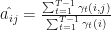
 is the probability of observing symbol
  in state j. The update rule becomes:

 to random values such that
  ,
,  and
and  . It is important to ensure that row probabilities add up to 1 and probabilities are not uniform as this may result in convergence to a local maximum.
 ,
,  , and
, and  and
and  , or the converged solution provides model parameters that are more likely for a given sequence of observations


