Solving ODEs Numerically

In this post we are going to look at two methods for approximating a solution to some ordinary differential equation. We will only consider the first order separable initial value problems. Here, the ‘first order’ means that the problem contains a first derivative only. The word ‘separable’ implies that the derivative can be separated from the derivative function (i.e. we can separate the derivative terms from the terms that do not involve derivatives). Finally, an initial value problem is a problem for which an initial condition is given, thus we have two starting values for x and y.

The following are examples of the types of problems we are considering:

$\frac{dy}{dx}=xy^{\frac{1}{3}}, y(1)=1$
$\frac{dy}{dx}=4x-3, y(0)=0$
$\frac{dy}{dx}=\cos{x}-3, y(0)=0$

The above examples contain expressions for the derivative of y(x). Thus, we are given the derivative, which is some function f() of x and y, and we are also given the initial value. This initial value is the value of x for which y(x) is already known. Please note that we do not know the exact expression for y(x), we just have the expression for the derivative of y w.r.t. x.

Solving a differential equation means finding the y(x). Numerical solutions to differential equations usually approximate the y(x) at some required point. So, a numerical solution does not produce an expression for y(x), it just approximates the value of y(x) at some point x. Given enough approximations, we should also be able to graph y(x) on some interval.

There are many types of approximations to differential equations. Here we will look at Euler’s and Runge-Kutta methods. Both methods are based on the Taylor series expansion. Since the function for the 1st derivative is known, this means that we have an equation for the slope to the curve y(x) makes on the (x,y) plane.

The basic definition of the first derivative is given by $\frac{dy}{dx}\approx \frac{\Delta}{\Delta x}= \frac{(y(x+h)-y(x))}{h}$ , which says that for some small change h, we can approximate the rate of change in y to the rate of change in x using this difference ratio. This can be rearranged to give us $y(x+h)$ . Thus: $y(x+h)=h[\frac{dy}{dx}]+y(x)$ . This expression can be used to solve a differential equation for some other value of x, since we can start with our initial condition, take a small step h, and iteratively approximate y(x). The smaller is the increment step, the better will be our approximation. This is the fundamental idea behind the Euler’s method.

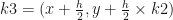
The Runge-Kutta method is a little bit more complex, but it is more accurate as well. This approach is building on the fact that $y(x+h)=h[\frac{dy}{dx}]+y(x)$ is an approximation that can be improved upon. In particular, the Runge-Kutta method is the 4th order approximation to the ordinary differential equation, thus we have: $y(x+h)=y(x)+h[\frac{1}{6}(k1+2\times k2+2\times k3+k4)]$ where
$k1=f(x,y)$ , $k2=f(x+ \frac{h}{2},y+ \frac{h}{2}\times k1)$ , $k3=(x+ \frac{h}{2},y+ \frac{h}{2}\times k2)$ and $k4=f(x+h,y+h\times k3)$ .

It comes as no surprise that the Runge-Kutta is more accurate than the Euler’s method since it is better at approximating the curve of y(x).

We will now look at the implementation of these two methods in C#. My code is given below. Note that I am following my usual coding style by making the individual solution classes to derive from an abstract InitialValue class. Most of the variables and functionality that is common to both method is contained within the parent class. The differential function is implemented as a delegate. Finally, I am also populating the metadata for the class constructors and the solution methods this time, as this is a good practice.

using System;
using System.Collections.Generic;

namespace DifferentialEquations
{

    abstract class InitialValue
    {
        internal delegate double DerivativeFunction(double x, double y);

        internal InitialValue(DerivativeFunction func, double initValX, double initValY, double solPoint)
        {
            givenFunction = func;
            this.initValX = initValX;
            this.initValY = initValY;
            this.solPoint = solPoint;
            CalcDistance();
        }

        internal double Delta
        {
            get
            {
               return delta;
            }
        }

        internal int Distance
        {
            get
            {
                return distance;
            }
        }

        //calculates absolute distance between the x point for required solution and the initial value of x
        private void CalcDistance()
        {
            double res = 0.0;
            
            if (this.initValX < 0 && this.solPoint < 0)
            {
                res = Math.Abs(Math.Min(this.initValX, this.solPoint) - Math.Max(this.initValX, this.solPoint));
            }
            else if (this.initValX > 0 && this.solPoint > 0)
            {
                res = Math.Max(this.initValX, this.solPoint) - Math.Min(this.initValX, this.solPoint);
            }
            else
            {
                res = Math.Abs(this.solPoint) + Math.Abs(this.initValX);
            }

            this.distance = (int)res;
        }

        internal abstract double[] SolveDifferentialEquation();

        protected DerivativeFunction givenFunction;
        private const double  delta=0.01;
        protected double initValX;
        protected double initValY;
        protected double solPoint;
        private int distance=0;

    }

    sealed class EulerMethod:InitialValue
    {

        /// <summary>
        /// Initialises the Euler method
        /// </summary>
        /// <param name="func">differential function to approximate</param>
        /// <param name="initValX">initial value for x</param>
        /// <param name="initValY">initial value for y</param>
        /// <param name="solPoint">solution point: value of x for which y=f(x) is required</param>
        internal EulerMethod(DerivativeFunction func, double initValX, double initValY, double solPoint):base(func,initValX, initValY, solPoint)
        {
            altDelta = base.Delta;
        }

        /// <summary>
        /// Initialises the Euler method
        /// </summary>
        /// <param name="func">differential function to approximate</param>
        /// <param name="initValX">initial value for x</param>
        /// <param name="initValY">initial value for y</param>
        /// <param name="solPoint">solution point: value of x for which y=f(x) is required</param>
        /// <param name="delta">alternative value for delta</param>
        internal EulerMethod(DerivativeFunction func, double initValX, double initValY, double solPoint, double delta)
            : base(func, initValX, initValY, solPoint)
        {
            //this check will not provide for all cases but good enough for demonstration
            if (delta < base.Distance)
                altDelta = delta;
            else
            {
                Console.WriteLine("Delta value too large. Using default delta of 0.01.");
                altDelta = base.Delta;
            }
        }

        /// <summary>
        /// Solves a differential equation using the Euler method
        /// </summary>
        /// <returns>y=f(x) solution at the required point of x</returns>
        internal override double[] SolveDifferentialEquation()
        {
            direction = (this.initValX < base.solPoint) ? true : false;

            //the position at index 0 will be taken by initial value
            int numPoints = (int)(base.Distance/ this.altDelta)+1;
            double[] solutionPoints = new double[numPoints];
            double x = this.initValX;

            solutionPoints[0] = this.initValY;

            for (int i = 0; i < numPoints-1; i++)
            {
                solutionPoints[i + 1] = solutionPoints[i] + altDelta * this.givenFunction(x, solutionPoints[i]);
                if (direction)
                    x = x + altDelta;
                else
                    x = x - altDelta;
            }
            Console.WriteLine("Euler Solution at x=: " + base.solPoint + " is " + solutionPoints.GetValue(numPoints - 1));
            return solutionPoints;
        }

        private bool direction;
        private double altDelta;
    }

    sealed class RungeKuttaMethod : InitialValue
    {
        /// <summary>
        /// Initialises the Runge-Kutta method
        /// </summary>
        /// <param name="func">differential function to approximate</param>
        /// <param name="initValX">initial value for x</param>
        /// <param name="initValY">initial value for y</param>
        /// <param name="solPoint">solution point: value of x for which y=f(x) is required</param>
        internal RungeKuttaMethod(DerivativeFunction func, double initValX, double initValY, double solPoint)
            : base(func, initValX, initValY, solPoint)
        {
            altDelta = base.Delta;
        }


        /// <summary>
        /// Initialises the Runge-Kutta method
        /// </summary>
        /// <param name="func">differential function to approximate</param>
        /// <param name="initValX">initial value for x</param>
        /// <param name="initValY">initial value for y</param>
        /// <param name="solPoint">solution point: value of x for which y=f(x) is required</param>
        /// <param name="delta">alternative delta value</param>
        internal RungeKuttaMethod(DerivativeFunction func, double initValX, double initValY, double solPoint, double delta)
            : base(func, initValX, initValY, solPoint)
        {
            //this check will not provide for all cases but good enough for demonstration
            if (delta < base.Distance)
                altDelta = delta;
            else
            {
                Console.WriteLine("Delta value too large. Using default delta of 0.01.");
                altDelta = base.Delta;
            }
        }

        /// <summary>
        /// Solves a differential equation using Runge-Kutta method
        /// </summary>
        /// <returns>y=f(x) solution at the required point of x</returns>
        internal override double[] SolveDifferentialEquation()
        {
            direction = (this.initValX < base.solPoint) ? true : false;

            //the position at index 0 will be taken by initial value
            int numPoints = (int)(base.Distance/ this.altDelta)+1;
            double[] solutionPoints = new double[numPoints];
            double x = this.initValX;
            double k1, k2, k3, k4 = this.initValY;
            double scale = 1.0/6.0;
            double increment = altDelta/2;

            solutionPoints[0] = this.initValY;

            for (int i = 0; i < numPoints - 1; i++)
            {
                k1 = this.givenFunction(x, solutionPoints[i]);
                k2 = this.givenFunction(x + increment, solutionPoints[i] + increment * k1);
                k3 = this.givenFunction(x + increment, solutionPoints[i] + increment * k2);
                k4 = this.givenFunction(x + altDelta, solutionPoints[i] + altDelta * k3);
                solutionPoints[i + 1] = solutionPoints[i] + altDelta*scale *(k1+2.0*k2+2.0*k3+k4);
                if (direction)
                    x = x + altDelta;
                else
                    x = x - altDelta;
            }
            Console.WriteLine("Runge-Kutta Solution at x=: "+base.solPoint+" is " + solutionPoints.GetValue(numPoints - 1));
            return solutionPoints;
        }

        private bool direction;
        private double altDelta;
    }

    
    class EntryPoint
    {
        static void Main(string[] args)
        {
            EulerMethod eu = new EulerMethod(DerivFunction, 0, 0,5);
            double[]resEU = eu.SolveDifferentialEquation();
            
            RungeKuttaMethod rk = new RungeKuttaMethod(DerivFunction, 0, 0,5);
            double[] resRK = rk.SolveDifferentialEquation();
            
            Console.ReadLine();
        }

        static double DerivFunction(double x, double y)
        {
            //double pow = (1.0 / 3.0);
            //return x * Math.Pow(y, pow);
            //return 14.0 * x - 3.0;
            return Math.Cos(x) - 3.0;
        }
    }
}

Below are the results for three initial value problems. Here the h increment is 0.01. The Runge-Kutta method provides a very good approximation.

Table 1
Differential Equation	Euler’s	Runge-Kutta	Exact Solution (at x=5)
$\frac{dy}{dx}=xy^{\frac{1}{3}}, y(1)=1$	26.8956	26.9999	27
$\frac{dy}{dx}=4x-3, y(0)=0$	159.6499	159.9999	160
$\frac{dy}{dx}=\cos{x}-3, y(0)=0$	-15.9553	-15.9589	-15.9589

Share this:

Like this:

Related