
In this post I will re-introduce and compare four well-known numerical integration techniques for approximating definite integrals of single-variable functions (e.g. polynomials). The compared techniques, in the order of least to the most accurate, are:
- Rectangle rule;
- Mid-point rule;
- Trapezoid rule;
- and Simpson’s rule;
Let me begin by an informal description of the idea behind numerical integration. All numerical integration involves approximating the area under the function’s curve. For example, Figure 1 is a plot of f(x)=2+cos(2*sqrt(x)) for x in the interval between 0 and 2. The area under the curve can be approximated in different ways. The simplest way is to break it up into many rectangles and compute their areas instead.
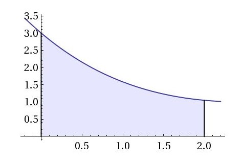
Figure 2 illustrates this simple ‘rectangle rule’ approach, where I only show three rectangles. Clearly, for this function, the rectangle rule approximation will overestimate the area. However, this is due to the fact that I began to break-up the area under the function’s curve left-to-right. This means that the area of the first rectangle is calculated by evaluating the functions at point x=a, and scaling by the distance between a and b, where b is the starting point of the next rectangle. Was I to start from left to right, as shown in Figure 3, I would have underestimated the area. If you are thinking that some kind of average of the two methods can give a more accurate approximation, you are absolutely correct. This, in fact, is what trapezoid-rule approximation does. Also, it is clear, that the more rectangles are used to break-up the area, the more accurate is the approximation.


It is probably a good time to formally define these numerical methods.
For any two adjacent points a and b, the area of a single rectangle is approximated as follows:
- Rectangle rule:
- Mid-point rule:
- Trapezoid rule:
- and Simpson’s rule:

](https://s0.wp.com/latex.php?latex=%5Cint_a%5Eb+%5C%21+f%28x%29+%5C%2C+%5Cmathrm%7Bd%7Dx+%5Capprox+%5Cfrac%7B1%7D%7B2%7D%5Bf%28a%29%2Bf%28b%29%5D%28b-a%29&bg=ffffff&fg=111111&s=0&c=20201002)
![\int_a^b \! f(x) \, \mathrm{d}x \approx \frac{1}{3}[f(a)+f(\frac{a+b}{2})+f(b)]](https://s0.wp.com/latex.php?latex=%5Cint_a%5Eb+%5C%21+f%28x%29+%5C%2C+%5Cmathrm%7Bd%7Dx+%5Capprox+%5Cfrac%7B1%7D%7B3%7D%5Bf%28a%29%2Bf%28%5Cfrac%7Ba%2Bb%7D%7B2%7D%29%2Bf%28b%29%5D&bg=ffffff&fg=111111&s=0&c=20201002)
Note that in the above definitions, I am assuming that b>a, and that my increment step is set to 1. Below I am providing a rather naïve implementation of these four numerical integration methods in C#:
using System;

//functionality to perform several types of single-variable function numerical integration
namespace NumericalIntegration
{
    public abstract class NumericalIntegration
    {
        public delegate double SingleVarFunction(double x);

        public NumericalIntegration(double from, double to, double steps, SingleVarFunction func)
        {
            this.fromPoint = from;
            this.toPoint = to;
            this.numSteps = steps;
            eps=0.0005;
            h = (toPoint - fromPoint) / (numSteps + 1.0);
            this.func=func;
        }

        public abstract double Integration();

        protected double fromPoint;
        protected double toPoint;
        protected SingleVarFunction func;
        protected double numSteps;
        protected double eps;
        protected double h;
    }

    public sealed class RectangleRule: NumericalIntegration
    {
        public RectangleRule(double from, double to, double steps, SingleVarFunction func)
            :base(from,to,steps,func)
        { }

        public override double Integration()
        {
            double a = fromPoint;
            double value = func(fromPoint);
            for (int i = 1; i <= numSteps; i++)
            {
                a = a + h;
                value += func(a);
            }
                return h*value;
        }
    }
public sealed class MidPointRule: NumericalIntegration
    {
        public MidPointRule(double from, double to, double steps, SingleVarFunction func)
            :base(from,to,steps,func)
        {}

        public override double Integration()
        {
            double a = fromPoint;
            double value = func((2.0 * fromPoint + h) / 2.0);
            for (int i = 1; i <= numSteps; i++)
            {
                a = a + h;
                value += func((2.0 * a + h) / 2.0);
            }
            return h * value;
        }
    }

    public sealed class TrapezoidRule: NumericalIntegration
    {
        public TrapezoidRule(double from, double to, double steps, SingleVarFunction func)
            : base(from, to, steps, func)
        {}
        public override double Integration()
        {
            double a = fromPoint;
            double value = (func(fromPoint)+func(fromPoint+h));
            for (int i = 1; i <= numSteps; i++)
            {
                a = a + h;
                value += (func(a) + func(a + h));
            }
            return 0.5 * h * value;
        }
    }

    public sealed class SimpsonRule: NumericalIntegration
    {
        public SimpsonRule(double from, double to, double steps, SingleVarFunction func)
            : base(from, to, steps, func)
        {
            h = (toPoint - fromPoint) / (numSteps * 2.0);
        }

        public override double Integration()
        {
            double valueEven = 0;
            double valueOdd = 0;

            for (int i = 1; i <= numSteps; i++)
            {
                valueOdd += func(fromPoint + this.h * (2.0 * i - 1));
                if (i <= numSteps-1)
                  valueEven += func(fromPoint + this.h * 2.0 * i);
            }
            return (func(fromPoint)+func(toPoint)+2.0*valueEven+4.0*valueOdd)*(this.h/3.0);
        }
    }
}
In summary, the code defines an abstract NumericalIntegration class which has two members: a delegate to point to the function over which we need to integrate, an abstract Integration method which must be overridden by the deriving classes. The assignment of the integration parameters occurs through the base class constructor. However, in case of the SimpsonRule class, I override the definition of h.
Please note that for the sake of this comparison, I will not be attempting to estimate the number of rectangles or partitions needed to achieve some convergence criterion. However, I am still declaring eps in the base class constructor, which can be used for this purpose.
Ok, so, let’s evaluate the Integration methods of each rule for the following functions and parameters: a=0, b=2, number of partitions = 8. Also, we’ll compare the performance on the following three functions:
- func1:
- func2:
- func3:


The last function’s lower bound is set to 0.1 instead of zero.
Table 1 summarises the results of each numerical integration rule. The last column shows the mathematical solution. Clearly, the Simpson’s rule is the most accurate here.
| func | rectangle | mid-point | trapezoid | Simpson’s | solution (to 6 d.p) |
|---|---|---|---|---|---|
| 1 | 3.68415 | 3.45633 | 3.46733 | 3.46000 | 3.46000 |
| 2 | 5.41971 | 5.51309 | 5.45394 | 5.49218 | 5.49946 |
| 3 | -0.50542 | -0.21474 | -0.25244 | -0.22756 | -0.22676 |
For the sake of completeness I provide the Main function code as well:
namespace TestNumericalIntegration
{
    using NumericalIntegration;

    class Program
    {
        static void Main(string[] args)
        {
            double from = 0.1;
            double to = 2.0;
            double steps = 20.0;

            RectangleRule ri = new RectangleRule(from, to, steps, funcToIntegrate);
            MidPointRule mi = new MidPointRule(from, to, steps, funcToIntegrate);
            TrapezoidRule ti = new TrapezoidRule(from, to, steps, funcToIntegrate);
            SimpsonRule si = new SimpsonRule(from, to, steps, funcToIntegrate);

            double[] res = { ri.Integration(), mi.Integration(), ti.Integration(), si.Integration() };
            foreach (double r in res)
                Console.WriteLine(r.ToString("F5", System.Globalization.CultureInfo.InvariantCulture));
            Console.ReadLine();
        }

        static double funcToIntegrate(double x)
        {
            //return 2.0+System.Math.Cos(2.0*System.Math.Sqrt(x));       //first function
            //return 2.0 + System.Math.Sin(2.0 * System.Math.Sqrt(x)); //second function
            return 0.4 * System.Math.Log(x*x);                       //third function

        }
    }
}
I hope you’ve found this useful. In my next post I will examine various approaches to numerical integration of multi-dimensional integrals.
